\(\mathbb P(\lambda\to\mu)=\frac{f^{\mu}}{(n+1)\,f^{\lambda}}\)Plancherel growth A Young diagram grown one box at a time with probability proportional to the dimension \(f^{\mu}\) of the resulting Specht module. Color shows hook length.
The math, in plain words
Imagine stacking boxes into a staircase, one at a time. At each step the box lands where it can, but some spots are "more popular" than others: a spot is favored in proportion to how many ways the final shape can be built (that count is \(f^\mu\)). Run this forever and a single, surprisingly stable limit shape appears. Randomness, left alone, draws a definite picture.
\(r=\cos(k\theta)\)Rose curves The family \(r=\cos(k\theta)\) with \(k\) drifting slowly through the rationals.
The math, in plain words
A rose is what you get by letting a point swing around the origin while its distance from the center oscillates, \(r=\cos(k\theta)\). If \(k\) is a whole number you get petals. If \(k=p/q\) is a fraction the curve closes only after \(q\) turns and the petals overlap into a lace. Here \(k\) slides slowly, so you watch simple arithmetic turn into geometry.
\(z_v\ge 4:\; z_v\to z_v-4,\ z_w\to z_w+1\)Abelian sandpile Grains dropped at the center of a grid topple when four or more accumulate; the order of toppling does not matter.
The math, in plain words
Drop grains of sand on one spot. When a pile holds four grains it collapses, giving one grain to each neighbor, which may in turn collapse. Remarkably, the final picture does not depend on the order in which piles are knocked over. That "order does not matter" rule is what makes the pattern so tidy, and it hides a beautiful commutative algebra.
\(i\mapsto k\,i \pmod N\)Times table on a circle Chords joining \(i\) to \(k\,i\) modulo the number of points \(N\), with \(k\) drifting from 2 to 10. At \(k=2\) the envelope is a cardioid; at \(k=3\), a nephroid.
The math, in plain words
Place \(N\) points on a circle and join each point \(i\) to the point \(k\,i\), counting around the circle. Nothing but multiplication, yet curves appear: for \(k=2\) a heart-shaped cardioid, for \(k=3\) a two-lobed nephroid. Straight lines can "envelope" a curve, just as many tangent lines trace the outline of a bend.
\(p_{t+1}=p_t+\tfrac{n}{n+3}\,(v-p_t)\)Chaos game A point repeatedly jumps part of the way toward a random vertex of a regular polygon. For 3, 4, 5 and 6 vertices, fractal structure emerges from pure randomness.
The math, in plain words
Pick a corner of a polygon at random and jump part of the way toward it. Repeat thousands of times. You would expect a smudge, yet a sharp fractal appears. The reason: every jump shrinks the picture toward a corner, so the pattern must look like a copy of itself made of smaller copies. Chance hides an exact structure.
\(z(t)=\sum_k c_k\,e^{ikt}\)Fourier epicycles A pentagram drawn by chained rotating circles, one per Fourier coefficient. Each pass adds more circles and the curve sharpens.
The math, in plain words
Ptolemy explained planets with circles riding on circles. It turns out that any closed curve can be drawn this way: a long chain of rotating arrows, each spinning at its own whole-number speed, adds up to a moving tip that traces the curve. The sum \(\sum c_k e^{ikt}\) is the Fourier idea: complicated motion is a blend of simple rotations.
\(\Delta\theta_0=10^{-3}\ \mathrm{rad}\)Double pendulums Eight double pendulums released with initial angles differing by \(10^{-3}\) radian. They move together at first, then part ways; every 22 seconds of simulated time the experiment restarts.
The math, in plain words
A single pendulum is predictable; hang a second one from its end and everything changes. The eight pendulums start almost identically, off by a thousandth of a radian, and for a while they dance together. Then they part ways completely. This sensitive dependence on starting conditions is what "chaos" means: the rules are exact, but long-term prediction is out of reach.
\(\begin{aligned}\dot x&=10(y-x)\\ \dot y&=x(28-z)-y\\ \dot z&=xy-\tfrac83 z\end{aligned}\)Lorenz attractor Two solutions of the Lorenz system starting \(10^{-3}\) apart. Both settle onto the same butterfly-shaped attractor, but soon end up on unrelated paths: the butterfly effect. The readout \(\Delta\) is their distance.
The math, in plain words
Edward Lorenz found these three simple equations while modeling the weather. Every path winds around two lobes like a butterfly, never repeating and never crossing itself. Two paths that start a hair apart stay on the same butterfly but soon follow different routes. The butterfly effect is not a metaphor, it is a theorem-sized fact about this system.
\(x_{n+1}=r\,x_n(1-x_n)\)Bifurcation diagram Long-run behavior of the logistic map \(x\mapsto rx(1-x)\) as \(r\) grows from 2.8 to 4: a fixed point, period doubling, then chaos with windows of order.
The math, in plain words
The rule \(x\mapsto rx(1-x)\) models a population: growth when small, crowding when large. For low \(r\) it settles to one value. Raise \(r\) and it starts alternating between two, then four, then eight values, doubling faster and faster until it never settles: chaos. Inside the chaos, calm windows return. The same pattern of doublings appears in many unrelated systems.
Interactive sketches
Click a thumbnail to open the sketch with its controls: sliders and buttons recompute everything live in your browser.
Circle packing in a rectangle
n equal circles are inflated and pushed apart inside a rectangle until no circle can grow. The radius found is a good packing (not always the optimal one), and touching circles are joined by segments.
\(\max r \ \text{s.t.}\ \|p_i-p_j\|\ge 2r,\ p_i\in[r,W-r]\times[r,H-r]\)
The math, in plain words
How big can \(n\) equal coins be if they must all fit in a box without overlapping? For a handful of coins the best arrangement is known, for many it is an open puzzle. The simulation inflates the coins and lets them push each other until they jam. The jammed state is a good packing, though not always the best one: many local optima, one global winner.
\(\max r \ \text{s.t.}\ \|p_i-p_j\|\ge 2r,\ p_i\in[r,W-r]\times[r,H-r]\)Circle packing in a rectangle n equal circles are inflated and pushed apart inside a rectangle until no circle can grow. The radius found is a good packing (not always the optimal one), and touching circles are joined by segments.
Apollonian circles
For two foci A and B, the locus |PA| = k·|PB| is a circle (red); the circles through A and B (blue) cut all of them at right angles. Together they form the bipolar grid.
Take two points A and B. The points whose distances to A and to B have a fixed ratio form a perfect circle, not an ellipse or anything else. The red circles from different ratios never touch, and the blue circles through A and B cross every red circle at exactly a right angle. Two families of circles, fitting together like a woven net.
\(\frac{|PA|}{|PB|}=k,\qquad R=\frac{2ck}{|k^2-1|}\)Apollonian circles For two foci A and B, the locus |PA| = k·|PB| is a circle (red); the circles through A and B (blue) cut all of them at right angles. Together they form the bipolar grid.
Lissajous figures
Two perpendicular oscillations with integer frequencies \(a\) and \(b\) and a phase shift \(\delta\). Rational ratios give closed curves; changing \(\delta\) makes the figure turn like a rotating ribbon.
\(x=A\sin(at+\delta),\quad y=B\sin(bt)\)
The math, in plain words
Make a point swing left-right at one speed and up-down at another. If the speeds are in a ratio of small whole numbers, like 3 to 2, the path closes into a neat loop. Shifting the phase makes the loop twist as if it were a 3-D ribbon turning. These are the curves an oscilloscope draws, and a visual way to "see" a musical interval.
\(x=A\sin(at+\delta),\quad y=B\sin(bt)\)Lissajous figures Two perpendicular oscillations with integer frequencies \(a\) and \(b\) and a phase shift \(\delta\). Rational ratios give closed curves; changing \(\delta\) makes the figure turn like a rotating ribbon.
Fourier epicycles
Draw any closed curve with the mouse or a finger; the discrete Fourier transform turns it into a chain of rotating circles whose tip retraces the drawing. Use fewer circles to see how the approximation degrades.
\(z(t)=\sum_{k=-m}^{m} c_k\,e^{ikt}\)
The math, in plain words
Any loop you draw can be rebuilt from circles. The computer measures how much of each spinning speed hides in your drawing (the discrete Fourier transform) and stacks one circle per speed. Big circles carry the rough shape, small ones add the sharp corners. Speech, music and images are compressed with exactly this idea: keep the big circles, drop the tiny ones.
\(z(t)=\sum_{k=-m}^{m} c_k\,e^{ikt}\)Fourier epicycles Draw any closed curve with the mouse or a finger; the discrete Fourier transform turns it into a chain of rotating circles whose tip retraces the drawing. Use fewer circles to see how the approximation degrades.
Mandelbrot and Julia sets
Left: the Mandelbrot set; click or drag to choose \(c\). Right: the Julia set of \(z^2 + c\) for that \(c\). Zoom with the slider and change the iteration limit.
\(z_{n+1}=z_n^2+c\)
The math, in plain words
Choose a number \(c\), start at 0 and repeat \(z\mapsto z^2+c\). Either the values stay bounded or they run away. The Mandelbrot set is the map of every \(c\) for which they stay. Each point of that map also has its own Julia set on the right: connected where \(c\) is inside, dust where \(c\) is outside. One tiny rule, endless detail.
\(z_{n+1}=z_n^2+c\)Mandelbrot and Julia sets Left: the Mandelbrot set; click or drag to choose \(c\). Right: the Julia set of \(z^2 + c\) for that \(c\). Zoom with the slider and change the iteration limit.
Möbius transformations of the Apollonian grid
A Möbius map sends circles to circles. Here it acts on the bipolar grid of Apollonian circles; change the parameters and watch the family bend but stay made of circles.
\(w=\frac{az+b}{cz+d},\quad ad-bc\neq 0\)
The math, in plain words
A Möbius map \(w=\frac{az+b}{cz+d}\) can stretch, rotate, shrink and flip the plane, but it never turns a circle into anything but a circle (a line counts as a circle through infinity). That is why the grid of circles bends yet keeps its character and its right-angle crossings. Möbius maps are the symmetries of the sphere's conformal geometry.
\(w=\frac{az+b}{cz+d},\quad ad-bc\neq 0\)Möbius transformations of the Apollonian grid A Möbius map sends circles to circles. Here it acts on the bipolar grid of Apollonian circles; change the parameters and watch the family bend but stay made of circles.
The chaos game
Pick a random vertex of a polygon and jump a fixed fraction of the way towards it, over and over. For the right fraction a fractal appears: the Sierpiński triangle, the Vicsek fractal and relatives.
\(p_{k+1}=p_k+r\,(v_{j}-p_k)\)
The math, in plain words
Pick a corner of a polygon at random and jump part of the way toward it. Repeat thousands of times. You would expect a smudge, yet a sharp fractal appears. The reason: every jump shrinks the picture toward a corner, so the pattern must look like a copy of itself made of smaller copies. Chance hides an exact structure.
\(p_{k+1}=p_k+r\,(v_{j}-p_k)\)The chaos game Pick a random vertex of a polygon and jump a fixed fraction of the way towards it, over and over. For the right fraction a fractal appears: the Sierpiński triangle, the Vicsek fractal and relatives.
The Collatz tree
Every number n leads to 1 under n ↦ n/2 (even) or 3n+1 (odd). The tree of all backward orbits from 1 is drawn up to a chosen depth, with turning angles you control.
Pick a number. If it is even, halve it; if odd, triple it and add one. Repeat. Everyone who has tried it ended at 1, but nobody can prove it always happens, and the problem is open since 1937. The tree shows every number that ends at 1 in a given number of steps, branching like a plant that no one fully understands.
\(n\mapsto\begin{cases}n/2 & n\text{ even}\\ 3n+1 & n\text{ odd}\end{cases}\)The Collatz tree Every number n leads to 1 under n ↦ n/2 (even) or 3n+1 (odd). The tree of all backward orbits from 1 is drawn up to a chosen depth, with turning angles you control.
Voronoi diagrams and Delaunay triangulations
Each site owns the cell of points closer to it than to any other site (Voronoi); joining sites whose cells touch gives the Delaunay triangulation, whose circumcircles contain no site. Drag, add or delete points, let them drift, or apply Lloyd's relaxation and watch the cells turn into a centroidal tessellation, almost hexagonal.
Scatter some towns on a map and give each house to the nearest town. The regions are the Voronoi cells, always convex polygons. Connect towns whose regions share a border and you get the Delaunay triangulation, which avoids skinny triangles as much as possible. Cell phone towers, crystal grains and animal territories all follow this pattern.
\(V(p_i)=\{x:\ \|x-p_i\|\le\|x-p_j\|\ \forall j\}\)Voronoi diagrams and Delaunay triangulations Each site owns the cell of points closer to it than to any other site (Voronoi); joining sites whose cells touch gives the Delaunay triangulation, whose circumcircles contain no site. Drag, add or delete points, let them drift, or apply Lloyd's relaxation and watch the cells turn into a centroidal tessellation, almost hexagonal.
Voronoi stippling of a photograph
Dots are moved to the centre of mass of their Voronoi cell, weighted by the brightness of the picture (Lloyd's algorithm), until the dots alone redraw the image. It starts with Einstein; upload your own photo (it never leaves your browser) or drop one onto the picture, then save the result as PNG or JPG.
Dots, nothing else. Each dot sits at the balance point of the patch of paper that is closer to it than to any other dot, weighted by how bright the photo is there. Repeating the balancing spreads dots densely where the image is dark and thinly where it is light, so the picture appears from points alone, like a newspaper photograph drawn by a mathematician.
\(x_i\leftarrow\frac{\int_{V_i} \rho(x)\,x\,dx}{\int_{V_i} \rho(x)\,dx}\)Voronoi stippling of a photograph Dots are moved to the centre of mass of their Voronoi cell, weighted by the brightness of the picture (Lloyd's algorithm), until the dots alone redraw the image. It starts with Einstein; upload your own photo (it never leaves your browser) or drop one onto the picture, then save the result as PNG or JPG.
Looping sketches
White and colour on black. Each one loops forever and carries a piece of mathematics; click to enlarge.
\(k=n\pi r^{2},\qquad k_{\mathrm{perc}}\approx 4.51,\qquad k_{\mathrm{conn}}\approx\ln n\)Random geometric graph 160 points wander on a torus and two are joined whenever they are closer than \(r\), while \(r\) slowly breathes in and out. Isolated points fade, small components get their own colour, and the giant component turns white at mean degree \(k = n\pi r^2 \approx 4.51\) (continuum percolation); the whole graph is connected only near \(k=\ln n\) (Penrose). The inset records the share of the largest component as r sweeps.
The math, in plain words
Scatter points at random and connect those that are close. With few connections per point you see only little islands; as the average number of neighbors passes about 4.5, a giant connected cluster suddenly appears (a phase transition, like water freezing). Near \(\ln n\) neighbors, nearly every point is attached. Networks switch from fragments to a whole very abruptly.
\((x,y)\mapsto(x+A\sin y,\;y),\qquad (x,y)\mapsto(x,\;y+A\sin x),\qquad \det=1\)Stirring and un-stirring 62,500 coloured particles on a torus are stirred by alternating shears, x ↦ x + A sin y and then y ↦ y + A sin x. Each shear preserves area, so the flow is incompressible and yet chaotic: the colour bands are stretched and folded into ever finer filaments. Every step is invertible, so the film then runs backwards and the original picture re-emerges exactly, as in G. I. Taylor's dye experiment.
The math, in plain words
Stirring coffee with a spoon mixes it, and that is what these shears do to the colored dots. But each shear preserves area and is perfectly reversible: run it backward and the original picture returns exactly. Mixing is not loss of information, only information hidden in fine folds. Disorder can be an exact, undoable rearrangement.
\(\dot\theta_i=\kappa\,\mathrm{Arg}\Big(e^{-i\theta_i}\sum_{j\sim i}e^{i\theta_j}\Big)+\sqrt{2D}\,\xi_i,\qquad \psi=\Big|\frac1n\sum_j e^{i\theta_j}\Big|\)Flocking: the Vicsek model 180 birds fly at constant speed and keep turning toward the average heading of their neighbours, against random noise of intensity \(D\). Colour is heading. As the noise sweeps down the flock suddenly locks into a common direction, a phase transition measured by the order parameter \(\psi\) in the inset; as it sweeps up the flock dissolves again.
The math, in plain words
Each bird follows one rule: look at your neighbors and turn toward their average heading, with a little random wobble. No leader, no plan. With little noise the whole flock locks into a common direction; with a lot, it dissolves into confusion. The number \(\psi\) between 0 and 1 measures how aligned the flock is, and it jumps from low to high as noise falls.
\(x_i=\frac{\int_{V_i}x\,\rho(x)\,dx}{\int_{V_i}\rho(x)\,dx},\qquad x_i(s)=(1-s)\,x_i^{E}+s\,x_{\sigma(i)}^{T}\)Stippling: Einstein and Tesla 18,000 dots, each at the centre of mass of its Voronoi cell under the brightness of a portrait (Lloyd's algorithm), so the dots alone redraw the photograph. Matching the two dot sets one-to-one by optimal transport lets every dot glide along a straight line from Einstein's place to Tesla's. The return trip uses the very same path, so the loop closes exactly. Halfway through, d3-delaunay computes live, in your browser, the Voronoi diagram of the moving dots on the way out and its dual, the Delaunay triangulation, on the way back.
The math, in plain words
Dots, nothing else. Each dot sits at the balance point of the patch of paper that is closer to it than to any other dot, weighted by how dark the photo is there. Repeating this spreads dots densely in dark areas and thinly in light ones, so a face emerges. The morph then slides each dot to a partner in the second portrait, with partners chosen so that the total distance walked stays as small as possible.
\(\Pr(\sigma_i\to-\sigma_i)=\min\bigl(1,e^{-\Delta E/T}\bigr),\qquad T_c=\frac{2}{\ln(1+\sqrt2)}\approx2.269\)The Ising model: cooling through Tc 25,600 spins, each up (orange) or down (blue), flip by the Metropolis rule: always if that lowers the energy, otherwise with probability \(e^{-\Delta E/T}\). The temperature cycles, and as it crosses the critical value \(T_c=2/\ln(1+\sqrt2)\approx2.269\) the random froth coarsens into huge domains and a net magnetization appears, then melts again on heating. The inset follows \(|m|\) against \(T\); the white curve is Onsager's exact result, \(\bigl(1-\sinh^{-4}(2/T)\bigr)^{1/8}\).
The math, in plain words
Every spin just wants to agree with its four neighbors, and heat keeps shaking them out of it. Hot, the picture is static; cold, one color wins the whole sheet. In between, at exactly one temperature, patches of every size appear at once, and the magnetization \(|m|\) switches on with infinite slope. Lars Onsager solved this exactly in 1944.
\(u_t=D_u\Delta u-uv^{2}+F(1-u),\quad v_t=D_v\Delta v+uv^{2}-(F+k)v\)Turing patterns: Gray–Scott Two chemicals diffuse and react on a torus: \(u\) is fed in at rate \(F\), \(v\) is removed at rate \(k\), and \(u+2v\to3v\). A uniform state loses stability to diffusion and spots, stripes and mazes bloom, as in Turing's 1952 paper on morphogenesis. The feed and kill rates travel once around the loop drawn in the inset, so the pattern keeps splitting, stretching and rearranging as the point crosses regimes.
The math, in plain words
Alan Turing showed in 1952 that two chemicals that diffuse at different speeds can turn a perfectly smooth mixture into spots and stripes, a possible recipe for animal coats. Here one chemical feeds another that eats it back, and nudging the two rates \(F\) and \(k\) a hair changes spots into worms into mazes.
Polynomial and matrix art
Pictures made of millions of roots or eigenvalues. Click a picture to open the sketch with its controls and explanation.
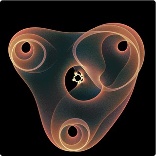
Art from the roots of polynomials Pick two random points on the unit circle, solve a degree-8 equation, and plot the eight roots; do it millions of times and a glowing, translucent figure appears. After the mathematical art of Simone Conradi.
Art from the roots of polynomials
Pick two random points on the unit circle, solve a degree-8 equation, and plot the eight roots; do it millions of times and a glowing, translucent figure appears. After the mathematical art of Simone Conradi.
The artist
This page is based on the mathematical art of Simone Conradi, who publishes his work at profconradi.github.io: computational pictures of polynomial roots and of patterns in the complex plane, and physics simulations, all written in Python (his site's tagline is “Where mathematics becomes visible”). On GitHub (profConradi) he shares notebooks on fractals, eigenvalue pictures (“eigenfish”), artificial life and other Python simulations, which makes this kind of picture part of a wider habit of looking at mathematics by computing it.
The image that inspired this sketch is signed “Simone Conradi, 2024” and prints its polynomial across the top. The idea, the polynomial and the overall look are his. The code on this page is my own re-implementation and the colours were matched by eye, not copied from his files, so small differences are expected. Please visit his page and look at the originals.
(The printed form has the middle coefficient as \(-500i\,t_1^3+500i\,t_1^2-500\,t_1+500i\); factoring out \(500i\) gives the form above, and \(1.5625=25/16\).) Every term has a factor \(x^2\), so \(P=x^2Q\) with
The double root at \(0\) is the same for every parameter, so it is dropped; the picture shows the eight roots of \(Q\). Write \(t_1=e^{i\alpha}\) and \(t_2=e^{i\beta}\): the parameters live on a torus \(\mathbb T^2=S^1\times S^1\), and each point \((\alpha,\beta)\) of it gives eight points of the plane. Two simple facts hold for all of them (I checked them numerically): \(Q\) has no \(x^7\) term, so the eight roots always have centre of mass \(0\); and their product is \(\tfrac{25/16}{16}=\tfrac{25}{256}\), so their geometric mean modulus is always \((25/256)^{1/8}\approx0.748\). Typically four roots are small (near \(0.2\)) and four are large (\(2\) to \(4\)): the small ones make the little ornament in the centre, the large ones make the big three-lobed shape.
The image is the set of all roots as the parameters range over the torus, drawn with a density. That set has a neat description. Solving \(Q(x)=0\) for \(t_2\) gives
So a point \(x\) of the plane is a root for some parameters exactly when \(|1+iR_{t_1}(x)|=1\) for some \(t_1\) on the circle, that is, when \(R_{t_1}(x)\) lies on the circle of radius \(1\) centred at \(i\). For a fixed \(t_1\) the roots therefore form a curve: the preimage of a circle under a rational map of degree \(8\). As \(t_1\) runs once around the circle the curve moves and sweeps out a region. The picture is the union of all these curves.
Why rings and holes
The map \((\alpha,\beta)\mapsto x\) goes from a surface (the torus, covered eight times by the root sheets) to the plane, so it fills regions rather than drawing curves. Where its derivative degenerates (a fold) the points of the torus on both sides of the fold are sent to the same side of a curve and pile up there: for a generic fold the density of dots grows like \(1/\sqrt{d}\), where \(d\) is the distance to the fold curve. That is the same mechanism that makes the bright lines (caustics) at the bottom of a coffee cup in sunlight, and it is what you see as the glowing rings and sharp edges. The dark holes are points \(x\) for which no choice of \((t_1,t_2)\) on the circles produces a root. Where several sheets overlap the density adds up, which gives the layered, translucent look.
How the picture is computed
Choose \(\alpha,\beta\) uniformly at random; set \(t_1=e^{i\alpha}\), \(t_2=e^{i\beta}\) and form \(A\) and \(B\).
Find the eight roots of \(Q\) with the Aberth–Ehrlich iteration, a simultaneous Newton method in which every approximation repels the others: with \(N_k=Q(z_k)/Q'(z_k)\), \[z_k\leftarrow z_k-\frac{N_k}{1-N_k\sum_{j\ne k}\frac{1}{z_k-z_j}}.\] Start on a circle and stop when every step is below \(10^{-11}\). It finds all roots at once and is much faster than building an eigenvalue problem for every sample. (Roots can also be computed as eigenvalues of the companion matrix, which is probably what a Python script would do with numpy.roots.)
Drop each root into a pixel grid. Instead of lighting one pixel, a root of weight \(1\) is shared between the four nearest pixels (bilinear weights). This acts like a much smaller dot and removes the blocky look of single-pixel histograms.
For every pixel keep three numbers: the total weight, and the sums of \(\cos\alpha\) and \(\sin\alpha\) of the parameters that produced the roots there (their direction is the local mean of \(t_1\)).
Tone map. After a light \(3\times3\) smoothing, the weight \(n\) becomes a brightness \(v=\bigl(\ln(1+n/p)/\ln(1+q/p)\bigr)^{\gamma}\), where \(p\) and \(q\) are low and high percentiles of the picture, so faint regions stay visible next to the glowing rings. Colour comes from a ramp teal → salmon → cream in \(v\), with the low-density fringes tinted blue or crimson according to the mean direction of \(t_1\). The ramp was matched by eye to colours sampled from Conradi's image, which is warmer than my first attempt.
Many threads (Web Workers) compute different random samples at the same time and send their partial pictures to the page, which adds them. One pair costs roughly the same as a few thousand arithmetic operations, so millions of pairs take from seconds to minutes depending on the computer.
Why millions of pairs? This is a Monte Carlo picture: the noise in a pixel falls like \(1/\sqrt{n}\), so four times as many pairs halve the grain. With a few hundred thousand pairs the interior looks sandy; with several million it becomes a smooth glow, and the fine structure of the rings appears. A larger canvas needs proportionally more points for the same smoothness, which is why the resolution and the number of pairs are separate controls.
Colours and HDR. Besides the paper, script and gradient schemes described below, the Colours menu has twelve ramps: the warm one tuned to Conradi’s image, my first teal-and-salmon one, ember, ice, aurora, dusk, gold, a viridis-like one, pastel and vivid hues from the colour source (\(t_1\), \(t_2\) or the index of the root), cream and white. If your screen and browser can show high dynamic range (for example the XDR screen of a MacBook Pro or an iPhone, in a browser that supports it), a checkbox appears: the picture is then drawn on a WebGPU canvas in extended range and the brightest ridges are multiplied, in linear light, by up to the chosen factor, so they glow brighter than the white of the page. The box is hidden when the browser does not report an HDR display and extended tone mapping; if you believe your device supports it, add ?hdr=1 to the address to force it. A saved PNG is always the standard (SDR) version.
Is it significant, or just a beautiful picture?
My honest answer: it is experimental art with real mathematics inside it, but I know of no theorem about this particular polynomial, and I do not know how it was found. The numbers \(500\) and \(25/16\) look hand-tuned: the large factor \(500\) makes the middle terms compete with the \(16x^8\) and constant terms at moduli where four roots are near \(0.2\) and four near \(3\), and small changes change the picture a lot (try the sliders). The most likely route is the one an experimenter would take: choose a family of polynomials with unimodular parameters, plot, adjust the coefficients, repeat.
Several real ideas are visible in it, though. Roots depend continuously on coefficients, so a torus of parameters is carried to a two-dimensional blob. Folds and the \(1/\sqrt{d}\) density are standard singularity theory (Whitney folds and cusps, the same caustics as in optics). The set of possible roots of a family of polynomials is exactly the question of “robust stability” in control theory (where can the roots go if the coefficients vary over a set?), and root pictures of structured families are an old mathematical tradition: the roots of all polynomials with small integer coefficients (John Baez's “The beauty of roots”), of Littlewood polynomials, or the eigenvalue pictures of random and structured matrices. Here the parameters are two angles, which is the smallest family that fills regions and still has folds you can follow by hand.
Things to try: set the zoom to about \(9\times\) to see the small ornament near the origin; click on the picture to recentre; change \(c\) and watch the holes move and merge; change \(s\) to see the shape inflate or collapse; compare “hue by \(t_1\)” with “hue by \(t_2\)” to see which parameter pushes a root where.
The constant term \(c\)
The slider for \(c\) (from \(0\) to \(500\), on a cubic scale so that small values are easy to reach, plus a box for the exact value) multiplies the last coefficient: \(Q(x)=16x^{8}+A\,x^{5}+B\,x^{4}+c/16\) (up to the factor \(16\) that was divided out). It controls the size of the central detail of the picture: a small \(c\) shrinks it and a large \(c\) enlarges it. The default \(c=1.5626\) is close to the \(25/16=1.5625\) of the printed image; the Python script below uses \(c=18.345\). For \(c=0\) the polynomial has a root of multiplicity four at \(0\), and the picture handles that case too.
Colours, the gradient tool and the graphics card
The paper scheme paints translucent pastel ink on a light background. The script scheme is the one of the Python script below: the hue is the angle of the first parameter (\(t_1\) or \(\alpha\)), the saturation is \(0.8\), and the brightness grows from \(0.2\) to \(1\) with the angle of the second parameter (\(t_2\) or \(\beta\)), on black. With my gradient you design the colours yourself: click the bar to add a colour stop, drag a stop to move it, change its colour with the colour box, and use the presets or Reverse as a start. The gradient can colour the density (dark where few roots fall, light where many do) or the colour source (the gradient is looped over a full turn, so a gradient whose last stop equals the first one has no seam). The state of the gradient travels in the Share link.
If your browser offers WebGPU, the box Use the graphics card moves the computation to the GPU. One GPU thread takes one pair of parameters and finds all the roots of that polynomial at once with the Aberth–Ehrlich iteration, \[z_k\leftarrow z_k-\frac{1}{\dfrac{p\,\prime(z_k)}{p(z_k)}-\displaystyle\sum_{j\ne k}\frac{1}{z_k-z_j}},\qquad k=1,\dots,n,\]and thousands of such threads run side by side, each for a different pair \((t_1,t_2)\). For the matrices the GPU uses a closed formula (the ring) or a Hessenberg–QR iteration (the other families). With the GPU on, the limits rise to \(2\times10^{8}\) samples and a resolution of \(2160\) pixels. The GPU works in 32-bit arithmetic, enough for a picture but not for a certified answer; the matrix family with non-normal Toeplitz blocks is so sensitive to rounding that it always runs on the CPU, in 64-bit. Untick the box to compare the two paths.
Try it yourself in Python
A self-contained script that draws a picture like this one on your own computer. It needs numpy and matplotlib (pip install numpy matplotlib), runs in a few seconds to a minute, and writes a PNG; change N, the colours, the background or the parameters and run it again.
# Root art: the roots of  P(x) = 16 x^10 + 500i (t2-1) x^7 + 500i (1 + i t1 + t1^2 - t1^3) x^6 + (25/16) x^2
# for many random pairs (t1, t2) on the unit circle, drawn as translucent pastel ink on paper.
# After the mathematical art of Simone Conradi (profconradi.github.io). Needs: pip install numpy matplotlib
import numpy as np
import matplotlib.pyplot as plt
from matplotlib.colors import hsv_to_rgb

N = 200_000          # number of pairs (t1, t2); try 20_000 first
SIZE = 1000          # pixels per side
C_CONST = 25 / 16    # the constant term of P; try 1.5626 or 18.345 (the picture's central detail grows with it)
HALF = 4.45          # the picture shows the square [-HALF, HALF]^2
PAPER = (0.957, 0.941, 0.902)   # background colour; try (0, 0, 0) for black

# Colour scheme: "paper" (translucent pastel ink on a light background), "script" (hue = angle of the first
# parameter, saturation 0.8, brightness 0.2 ... 1 from the second angle, on black) or "gradient" (your own colours below)
SCHEME = "paper"
GRADIENT = [(0.0, "#05030f"), (0.25, "#3a0f6b"), (0.5, "#c2185b"), (0.75, "#ff8a3d"), (1.0, "#fff3c4")]   # (position 0..1, colour)
GRADIENT_FOR = "density"   # "density" (dark = few roots) or "source" (the gradient is looped over the colour source; make the last colour equal the first)

rng = np.random.default_rng(1)
a1, a2 = rng.random(N) * 2 * np.pi, rng.random(N) * 2 * np.pi
t1, t2 = np.exp(1j * a1), np.exp(1j * a2)

# P = x^2 * Q, with Q of degree 8; make Q monic and take the eigenvalues of its companion matrix
c5 = 500j * (t2 - 1) / 16                       # coefficient of x^5
c4 = 500j * (1 + 1j * t1 + t1**2 - t1**3) / 16   # coefficient of x^4
c0 = np.full(N, C_CONST / 16, dtype=complex)   # constant term
C = np.zeros((N, 8, 8), dtype=complex)
C[:, 1:, :-1] = np.eye(7)                        # ones below the diagonal
C[:, 0, 2] = -c5                                 # first row: minus the coefficients of x^7 ... x^0
C[:, 0, 3] = -c4
C[:, 0, 7] = -c0
roots = np.linalg.eigvals(C)                     # shape (N, 8); the other two roots of P are 0

# colour of each root: its hue is the angle of t1 (use a2 or the root index for other looks)
hue = np.repeat(a1 / (2 * np.pi), 8)
x, y = roots.real.ravel(), roots.imag.ravel()

# histograms: how many roots per pixel, and the average hue direction (cos and sin) per pixel
rng_ = [[-HALF, HALF], [-HALF, HALF]]
kw = dict(bins=SIZE, range=rng_)
n, _, _ = np.histogram2d(y, x, **kw)
cs, _, _ = np.histogram2d(y, x, weights=np.cos(2 * np.pi * hue), **kw)
sn, _, _ = np.histogram2d(y, x, weights=np.sin(2 * np.pi * hue), **kw)
un, _, _ = np.histogram2d(y, x, weights=np.repeat(a2 / (2 * np.pi), 8), **kw)   # mean of the second angle, for the script colours

# tone map: logarithm of the density, scaled by a high percentile, then alpha-composite ink over the paper
dens = np.log1p(n / max(np.percentile(n[n > 0], 6), 1e-9))
v = np.clip(dens / np.percentile(dens[n > 0], 99.7), 0, 1)
alpha = np.clip(0.9 * v**0.55, 0, 1)[..., None]
h = (np.arctan2(sn, cs) / (2 * np.pi)) % 1
conc = np.clip(np.hypot(cs, sn) / np.maximum(n, 1) * 1.5 + 0.3, 0, 1)
ink = hsv_to_rgb(np.dstack([h, 0.78 * conc, np.full_like(h, 0.93)]))
if SCHEME == "paper":
    img = np.array(PAPER) * (1 - alpha) + ink * alpha
elif SCHEME == "script":
    m = np.maximum(n, 1)
    bright = 0.2 + 0.8 * np.clip(un / m, 0, 1)
    col = hsv_to_rgb(np.dstack([h, np.full_like(h, 0.8), bright]))
    a2_ = np.clip(v**0.6, 0, 1)[..., None]
    img = col * a2_                                  # on black
else:
    from matplotlib.colors import to_rgb
    pos = np.array([p for p, _ in GRADIENT]); cols = np.array([to_rgb(c) for _, c in GRADIENT])
    lut = lambda t: np.stack([np.interp(t, pos, cols[:, k]) for k in range(3)], axis=-1)
    if GRADIENT_FOR == "density":
        img = lut(v)
    else:
        img = lut(h) * alpha + np.array(PAPER) * (1 - alpha)

plt.figure(figsize=(8, 8))
plt.imshow(img[::-1], extent=[-HALF, HALF, -HALF, HALF])   # [::-1]: imaginary axis pointing up
plt.axis("off")
plt.savefig("root_art.png", dpi=150, bbox_inches="tight", pad_inches=0)
print("saved root_art.png")
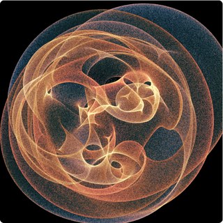
Art from the eigenvalues of matrices Two random angles define a complex matrix; compute its eigenvalues, plot them, and repeat millions of times. Four families of matrices, from a ring with gain and loss to random tori, and a button to surprise you.
Art from the eigenvalues of matrices
Two random angles define a complex matrix; compute its eigenvalues, plot them, and repeat millions of times. Four families of matrices, from a ring with gain and loss to random tori, and a button to surprise you.
What is plotted
This page uses the same recipe as the root picture, with matrices instead of a polynomial. Two angles \(\alpha,\beta\) are drawn at random; they define an \(N\times N\) complex matrix \(M(\alpha,\beta)\) (with \(N\) from \(4\) to \(48\) depending on the family and the slider); its \(N\) eigenvalues are computed and each is added as a faint dot to a picture of the complex plane. Millions of matrices later, the dots have drawn the region that the spectrum sweeps out as the two angles go around the torus.
Roots of polynomials and eigenvalues of matrices are the same thing seen from two sides: the eigenvalues of \(M\) are the roots of the characteristic polynomial \(\det(\lambda I-M)\), and the roots of a monic polynomial are the eigenvalues of its companion matrix. So the previous page is a special case. What is new here is that the matrices have structure (a ring, a band, a random torus, a companion matrix), and that their characteristic polynomials have a large degree, with coefficients that depend on \(\alpha,\beta\) in a very special way.
To fill regions of the plane the matrices must be non-normal. Hermitian matrices have real eigenvalues and unitary ones have eigenvalues on the unit circle, so their pictures are a segment or a circle; a generic complex matrix has eigenvalues that wander over the plane.
The four families
1. Non-Hermitian SSH ring with gain and loss. A ring of \(2c\) sites (\(c\) cells of two sites). Inside a cell the hopping is \(v\); between cells it is \(w\,e^{i\beta}\), a complex number; the sites alternately carry \(+i\gamma\) (gain) and \(-i\gamma\) (loss); and the bond that closes the ring carries an extra phase \(e^{\mp i\alpha}\), a magnetic flux through the ring. This is the Su–Schrieffer–Heeger chain, a textbook model of one-dimensional topological physics, with balanced gain and loss added, as studied in non-Hermitian physics. It has an exact solution: the \(2c\) eigenvalues are \[E=\pm\sqrt{\,v^{2}-\gamma^{2}+w^{2}e^{2i\beta}+2vw\,e^{i\beta}\cos k\,},\qquad k=\frac{2\pi m+\alpha}{c},\quad m=0,\dots,c-1\] (I checked this against the numerical eigenvalues to \(10^{-14}\)). So the picture is, up to the finite number of values of \(k\), the image of the torus \((k,\beta)\) under a simple explicit map: that is why it is crisp, with sharp folds and two cusp-shaped holes.
2. Banded Toeplitz matrix. A matrix with constant diagonals: \(1\) above the main diagonal, \(\sigma e^{i\beta}\) just below it and \(\rho e^{i\alpha}\) two places below it. Its symbol is \(a(z)=z+\sigma e^{i\beta}z^{-1}+\rho e^{i\alpha}z^{-2}\). The curve \(a(e^{i\theta})\) is the spectrum of the corresponding periodic (circulant) matrix, but the eigenvalues of the finite matrices do not follow it: as \(N\) grows they accumulate on a set of arcs (Schmidt–Spitzer, 1960), where two of the three roots of \(z^3-\lambda z^2+\sigma e^{i\beta}z+\rho e^{i\alpha}=0\) have equal modulus. Sweeping the two angles moves the arcs and paints the region between them.
3. Random torus. \(M=A_0+e^{i\alpha}A_1+e^{i\beta}A_2\), where \(A_0,A_1,A_2\) are fixed random complex matrices (Gaussian entries, a chosen fraction nonzero, scaled by \(1/\sqrt{N\,\text{density}}\)). For \(N=4\) this is a four-root cousin of the polynomial picture. Every value of the seed gives different matrices and therefore a different picture; the “Surprise me” button picks a family, parameters, seed and palette at random.
4. Companion matrix of a chirped polynomial. The polynomial \(x^N+\sum_{k\lt N}e^{i(\alpha k+\beta k^{p})}x^k\) has coefficients of modulus \(1\) whose phases form a “chirp” (linear plus a power of \(k\), \(p=2\) by default). Its roots are the eigenvalues of the companion matrix, with ones below the diagonal and the negated coefficients in the last column. For large \(N\) the roots of polynomials with bounded coefficients crowd near the unit circle (Erdős–Turán type results); here the two phase parameters decide how they spread around it.
How it is computed
Draw \(\alpha,\beta\) uniformly, build the \(N\times N\) complex matrix.
Compute all eigenvalues with my own complex QR algorithm: balance the matrix (diagonal scaling by powers of two, which tames very non-normal matrices), reduce it to Hessenberg form with Householder reflections, then run shifted QR iterations (Wilkinson shift, Givens rotations in complex arithmetic) with deflation. Cost grows like \(N^3\). I compared it with numpy on random, Toeplitz and ring matrices up to \(48\times48\): the eigenvalues agree to better than \(10^{-12}\).
Splat each eigenvalue into the density picture with bilinear weights, add the partial pictures of the worker threads, tone-map, colour (same engine and palettes as the root page).
The colour source can be \(\alpha\), \(\beta\), or the index of the eigenvalue in the computed list (for the ring and polynomial families the index follows the order of the computed list, so this colours by “which eigenvalue”).
HDR. If your screen and browser can show high dynamic range, a checkbox appears: the picture is then drawn on a WebGPU canvas in extended range and the brightest ridges are multiplied, in linear light, by up to the chosen factor, so they glow brighter than the white of the page. The box is hidden when the browser does not report an HDR display and extended tone mapping; if you believe your device supports it, add ?hdr=1 to the address to force it. A saved PNG is always the standard (SDR) version.
Is it significant, or just beautiful?
These pictures prove nothing, and the four families are my own choice; I have not seen the code behind Conradi's eigenvalue pictures (the “eigenfish” notebooks on his GitHub), so I make no claim about how his are made. But the mathematics under them is real and active. Spectra of non-normal and non-Hermitian matrices are central in numerical analysis (pseudospectra: Trefethen and Embree, Spectra and Pseudospectra), in the physics of open and lossy systems (optical and electronic structures with gain and loss, where Hermitian quantum mechanics no longer applies and the spectrum is complex), and in random matrix theory (a Gaussian matrix with entries of variance \(1/N\) has eigenvalues spread uniformly in the unit disk as \(N\to\infty\), the circular law). The Toeplitz family shows a classical fact that surprises newcomers: the eigenvalues of the finite sections do not approach the symbol curve.
The two-parameter sweep adds one more idea: an eigenvalue is a continuous function of the parameters, so the torus of angles is mapped onto regions of the plane, whose edges are folds where the eigenvalues crowd together (the same caustic mechanism as on the root page, with density growing like \(1/\sqrt{d}\) at a generic fold).
Things to try: in family 1 raise the gain and loss \(\gamma\) from \(0\) and watch the two holes open and close; in family 2 set \(\rho=0\) and then raise it; in family 3 press “Restart” with different seeds, or raise \(N\) to see the picture approach a disk-like blob; use the zoom on the sharp inner edges; try the HDR box on an HDR screen.
Colours, the gradient tool and the graphics card
The paper scheme paints translucent pastel ink on a light background. The script scheme is the one of the Python script below: the hue is the angle of the first parameter (\(t_1\) or \(\alpha\)), the saturation is \(0.8\), and the brightness grows from \(0.2\) to \(1\) with the angle of the second parameter (\(t_2\) or \(\beta\)), on black. With my gradient you design the colours yourself: click the bar to add a colour stop, drag a stop to move it, change its colour with the colour box, and use the presets or Reverse as a start. The gradient can colour the density (dark where few roots fall, light where many do) or the colour source (the gradient is looped over a full turn, so a gradient whose last stop equals the first one has no seam). The state of the gradient travels in the Share link.
If your browser offers WebGPU, the box Use the graphics card moves the computation to the GPU. One GPU thread takes one pair of parameters and finds all the roots of that polynomial at once with the Aberth–Ehrlich iteration, \[z_k\leftarrow z_k-\frac{1}{\dfrac{p\,\prime(z_k)}{p(z_k)}-\displaystyle\sum_{j\ne k}\frac{1}{z_k-z_j}},\qquad k=1,\dots,n,\]and thousands of such threads run side by side, each for a different pair \((t_1,t_2)\). For the matrices the GPU uses a closed formula (the ring) or a Hessenberg–QR iteration (the other families). With the GPU on, the limits rise to \(2\times10^{8}\) samples and a resolution of \(2160\) pixels. The GPU works in 32-bit arithmetic, enough for a picture but not for a certified answer; the matrix family with non-normal Toeplitz blocks is so sensitive to rounding that it always runs on the CPU, in 64-bit. Untick the box to compare the two paths.
Try it yourself in Python
A self-contained script that draws a picture like this one on your own computer. It needs numpy and matplotlib (pip install numpy matplotlib), runs in a few seconds to a minute, and writes a PNG; change N, the colours, the background or the parameters and run it again.
# Eigenvalue art: the eigenvalues of a complex matrix that depends on two angles (alpha, beta),
# drawn for many random angle pairs. Two families: "rand" (random sparse matrices) and "ssh" (a ring with gain and loss).
# Needs: pip install numpy matplotlib
import numpy as np
import matplotlib.pyplot as plt
from matplotlib.colors import hsv_to_rgb

FAMILY = "rand"      # "rand" or "ssh"
N = 100_000          # number of angle pairs; try 10_000 first
SIZE = 1000
PAPER = (0.957, 0.941, 0.902)

# Colour scheme: "paper" (translucent pastel ink on a light background), "script" (hue = angle of the first
# parameter, saturation 0.8, brightness 0.2 ... 1 from the second angle, on black) or "gradient" (your own colours below)
SCHEME = "paper"
GRADIENT = [(0.0, "#05030f"), (0.25, "#3a0f6b"), (0.5, "#c2185b"), (0.75, "#ff8a3d"), (1.0, "#fff3c4")]   # (position 0..1, colour)
GRADIENT_FOR = "density"   # "density" (dark = few roots) or "source" (the gradient is looped over the colour source; make the last colour equal the first)

rng = np.random.default_rng(7)
al, be = rng.random(N) * 2 * np.pi, rng.random(N) * 2 * np.pi

if FAMILY == "rand":
    # M(alpha, beta) = A0 + e^{i alpha} A1 + e^{i beta} A2 with three fixed random sparse 6 x 6 matrices
    n = 6
    A = [(rng.standard_normal((n, n)) + 1j * rng.standard_normal((n, n))) * (rng.random((n, n)) < 0.6) for _ in range(3)]
    M = A[0] + np.exp(1j * al)[:, None, None] * A[1] + np.exp(1j * be)[:, None, None] * A[2]
    HALF = 3.4
else:
    # non-Hermitian SSH ring: hopping v inside a cell, w e^{i beta} between cells, gain/loss +-i*gamma, twist alpha
    cells, v, w, gam = 12, 1.0, 1.6, 0.8
    n = 2 * cells
    M = np.zeros((N, n, n), dtype=complex)
    for j in range(n - 1):
        h = v if j % 2 == 0 else w * np.exp(1j * be)
        M[:, j, j + 1] = h
        M[:, j + 1, j] = h
    M[:, 0, n - 1] += w * np.exp(1j * (be - al))
    M[:, n - 1, 0] += w * np.exp(1j * (be + al))
    M[:, np.arange(n), np.arange(n)] += np.where(np.arange(n) % 2 == 0, 1j * gam, -1j * gam)
    HALF = v + w + gam + 0.2

ev = np.linalg.eigvals(M)                        # shape (N, n)
hue = np.repeat(al / (2 * np.pi), n)             # hue = the angle alpha
x, y = ev.real.ravel(), ev.imag.ravel()

kw = dict(bins=SIZE, range=[[-HALF, HALF], [-HALF, HALF]])
cnt, _, _ = np.histogram2d(y, x, **kw)
cs, _, _ = np.histogram2d(y, x, weights=np.cos(2 * np.pi * hue), **kw)
sn, _, _ = np.histogram2d(y, x, weights=np.sin(2 * np.pi * hue), **kw)
un, _, _ = np.histogram2d(y, x, weights=np.repeat(be / (2 * np.pi), n), **kw)   # mean of the second angle, for the script colours

dens = np.log1p(cnt / max(np.percentile(cnt[cnt > 0], 6), 1e-9))
v_ = np.clip(dens / np.percentile(dens[cnt > 0], 99.7), 0, 1)
alpha = np.clip(0.9 * v_**0.55, 0, 1)[..., None]
h = (np.arctan2(sn, cs) / (2 * np.pi)) % 1
conc = np.clip(np.hypot(cs, sn) / np.maximum(cnt, 1) * 1.5 + 0.3, 0, 1)
ink = hsv_to_rgb(np.dstack([h, 0.78 * conc, np.full_like(h, 0.93)]))
if SCHEME == "paper":
    img = np.array(PAPER) * (1 - alpha) + ink * alpha
elif SCHEME == "script":
    m = np.maximum(cnt, 1)
    bright = 0.2 + 0.8 * np.clip(un / m, 0, 1)
    col = hsv_to_rgb(np.dstack([h, np.full_like(h, 0.8), bright]))
    a2_ = np.clip(v_**0.6, 0, 1)[..., None]
    img = col * a2_                                  # on black
else:
    from matplotlib.colors import to_rgb
    pos = np.array([p for p, _ in GRADIENT]); cols = np.array([to_rgb(c) for _, c in GRADIENT])
    lut = lambda t: np.stack([np.interp(t, pos, cols[:, k]) for k in range(3)], axis=-1)
    if GRADIENT_FOR == "density":
        img = lut(v_)
    else:
        img = lut(h) * alpha + np.array(PAPER) * (1 - alpha)

plt.figure(figsize=(8, 8))
plt.imshow(img[::-1], extent=[-HALF, HALF, -HALF, HALF])
plt.axis("off")
plt.savefig("eigen_art.png", dpi=150, bbox_inches="tight", pad_inches=0)
print("saved eigen_art.png")
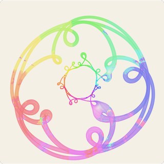
Roots of a degree-11 family After Simone Conradi's 2025 piece: two angles, eleven roots per pair, millions of pairs, in translucent pastel ink on paper.
Roots of a degree-11 family
After Simone Conradi's 2025 piece: two angles, eleven roots per pair, millions of pairs, in translucent pastel ink on paper.
The artist
The polynomial and the style of this picture come from a 2025 piece by Simone Conradi (profconradi.github.io), whose image prints the polynomial on top and plots its roots for many pairs of parameters on the unit circle, in translucent pastel colours on a cream background. I wrote the code myself from the polynomial printed on his image; it is a recreation in the same spirit, not his program, and the colours are not identical: his ribbons each have a colour of their own, while here the colour of a root comes from a label that follows the root as \(t_1\) goes around, so a ribbon can change colour where roots swap labels. Full credit for the design and for the family of polynomials goes to him. Choose “paper” in the Colours menu for this look, and pick another background if you like.
The polynomial
For two unimodular parameters \(t_1=e^{i\alpha}\) and \(t_2=e^{i\beta}\), the sketch solves \(P(x)=0\) with
Only two coefficients move: the one of \(x^9\) travels around a circle of radius \(|d_9|\approx 0.55\) as \(t_2\) goes around, and the one of \(x^7\) traces the closed curve \(q(e^{i\alpha})\), a trigonometric polynomial of degree \(5\) whose size is of the order of \(20\). The other nine coefficients are fixed and are all fourth roots of unity (\(\pm1,\pm i\)). So, unlike the first sketch, there is a large constant background and a strong, winding perturbation in the middle of the polynomial.
How it is computed
Each worker draws \((\alpha,\beta)\) at random, evaluates the two moving coefficients, divides the polynomial by its leading coefficient \(-i\) (which makes it monic), and finds all eleven roots with the Aberth–Ehrlich iteration, a Newton method that makes the approximations repel each other and therefore converges to all roots at once. To give every root a label, a sweep starts from the roots at \(t_1=t_2=1\) (labelled by decreasing modulus), walks \(t_2\) to a random point of the circle and then takes \(t_1\) once around, restarting the iteration from the previous roots at each small step. Each root is then splatted, with bilinear weights, into three histograms (weight, and the sum of \(\cos\) and \(\sin\) of a hue angle); the page tone-maps them exactly as in the first sketch, and the palettes, resolution, zoom, HDR and the “colour by” menu work the same way. Colouring by the index of the root shows how the eleven branches of the algebraic function \(x(t_1,t_2)\) are organised; colouring by \(t_1\) or \(t_2\) shows which parameter is responsible for each part of the picture.
What to look for
The picture is the projection to the plane of a two-dimensional surface in \(\mathbb C\): the union of the eleven root branches over the torus \((t_1,t_2)\). Because \(|d_9|\) is small, changing \(t_2\) only nudges each root a little, so the surface is a thin ribbon: each tube you see is the curve traced by a root as \(t_1\) goes once around the circle, thickened by the motion in \(t_2\). The small ring with five loops near the centre is the signature of \(q\) winding five times around the circle; the large loops are other branches, which \(q\) throws far from the origin. Where the ribbon folds over itself the density builds up and the picture darkens or brightens. Try colouring by \(t_2\) to see the ribbon's width, by the root index to separate the eleven branches, zooming into the loops, and increasing the pairs to a few million for a smooth image. I make no claim about the meaning of this particular family beyond what the picture shows; it is simply a beautiful one to look at.
Colours, the gradient tool and the graphics card
The paper scheme paints translucent pastel ink on a light background. The script scheme is the one of the Python script below: the hue is the angle of the first parameter (\(t_1\) or \(\alpha\)), the saturation is \(0.8\), and the brightness grows from \(0.2\) to \(1\) with the angle of the second parameter (\(t_2\) or \(\beta\)), on black. With my gradient you design the colours yourself: click the bar to add a colour stop, drag a stop to move it, change its colour with the colour box, and use the presets or Reverse as a start. The gradient can colour the density (dark where few roots fall, light where many do) or the colour source (the gradient is looped over a full turn, so a gradient whose last stop equals the first one has no seam). The state of the gradient travels in the Share link.
If your browser offers WebGPU, the box Use the graphics card moves the computation to the GPU. One GPU thread takes one pair of parameters and finds all the roots of that polynomial at once with the Aberth–Ehrlich iteration, \[z_k\leftarrow z_k-\frac{1}{\dfrac{p\,\prime(z_k)}{p(z_k)}-\displaystyle\sum_{j\ne k}\frac{1}{z_k-z_j}},\qquad k=1,\dots,n,\]and thousands of such threads run side by side, each for a different pair \((t_1,t_2)\). For the matrices the GPU uses a closed formula (the ring) or a Hessenberg–QR iteration (the other families). With the GPU on, the limits rise to \(2\times10^{8}\) samples and a resolution of \(2160\) pixels. The GPU works in 32-bit arithmetic, enough for a picture but not for a certified answer; the matrix family with non-normal Toeplitz blocks is so sensitive to rounding that it always runs on the CPU, in 64-bit. Untick the box to compare the two paths.
Try it yourself in Python
A self-contained script that draws a picture like this one on your own computer. It needs numpy and matplotlib (pip install numpy matplotlib), runs in a few seconds to a minute, and writes a PNG; change N, the colours, the background or the parameters and run it again.
# Degree-11 root art, after the 2025 image by Simone Conradi (profconradi.github.io):
# -i x^11 + x^10 + (t2 (-0.537-0.114i) - 0.571+0.414i) x^9 + x^8 + q(t1) x^7 + i x^6 - i x^5 + x^4 + i x^3 - x^2 + i x - i,
# q(t) = t^5 (-18.8-3.25i) + t^4 (-4.85+14i) + t^3 (5.81+12.6i) + t^2 (-8.74+4.29i) + t (5.81+0.687i) - 2.44+3.23i,   |t1| = |t2| = 1.
# Needs: pip install numpy matplotlib
import numpy as np
import matplotlib.pyplot as plt
from matplotlib.colors import hsv_to_rgb

N = 100_000          # number of pairs (t1, t2); try 10_000 first
SIZE = 1000
HALF = 3.0
PAPER = (0.957, 0.941, 0.902)

# Colour scheme: "paper" (translucent pastel ink on a light background), "script" (hue = angle of the first
# parameter, saturation 0.8, brightness 0.2 ... 1 from the second angle, on black) or "gradient" (your own colours below)
SCHEME = "paper"
GRADIENT = [(0.0, "#05030f"), (0.25, "#3a0f6b"), (0.5, "#c2185b"), (0.75, "#ff8a3d"), (1.0, "#fff3c4")]   # (position 0..1, colour)
GRADIENT_FOR = "density"   # "density" (dark = few roots) or "source" (the gradient is looped over the colour source; make the last colour equal the first)
COLOR_BY = "index"   # "index" (position of the root in the eigenvalue list), "t1" or "t2"

rng = np.random.default_rng(2)
a1, a2 = rng.random(N) * 2 * np.pi, rng.random(N) * 2 * np.pi
t1, t2 = np.exp(1j * a1), np.exp(1j * a2)

q = (t1**5 * (-18.8 - 3.25j) + t1**4 * (-4.85 + 14j) + t1**3 * (5.81 + 12.6j)
     + t1**2 * (-8.74 + 4.29j) + t1 * (5.81 + 0.687j) - 2.44 + 3.23j)
c9 = t2 * (-0.537 - 0.114j) - 0.571 + 0.414j
fixed = {11: -1j, 10: 1, 8: 1, 6: 1j, 5: -1j, 4: 1, 3: 1j, 2: -1, 1: 1j, 0: -1j}   # coefficients that do not move
coef = np.zeros((N, 12), dtype=complex)           # column k holds the coefficient of x^(11-k)
for deg, c in fixed.items():
    coef[:, 11 - deg] = c
coef[:, 11 - 9] = c9
coef[:, 11 - 7] = q
coef = coef / coef[:, :1]                         # divide by the leading coefficient -i: the polynomial becomes monic

C = np.zeros((N, 11, 11), dtype=complex)          # companion matrices
C[:, 1:, :-1] = np.eye(10)
C[:, 0, :] = -coef[:, 1:]
roots = np.linalg.eigvals(C)                      # shape (N, 11)

if COLOR_BY == "t1":
    hue = np.repeat(a1 / (2 * np.pi), 11)
elif COLOR_BY == "t2":
    hue = np.repeat(a2 / (2 * np.pi), 11)
else:
    hue = np.tile(np.arange(11) / 11, N)
x, y = roots.real.ravel(), roots.imag.ravel()

kw = dict(bins=SIZE, range=[[-HALF, HALF], [-HALF, HALF]])
cnt, _, _ = np.histogram2d(y, x, **kw)
cs, _, _ = np.histogram2d(y, x, weights=np.cos(2 * np.pi * hue), **kw)
sn, _, _ = np.histogram2d(y, x, weights=np.sin(2 * np.pi * hue), **kw)
un, _, _ = np.histogram2d(y, x, weights=np.repeat(a2 / (2 * np.pi), 11), **kw)   # mean of the second angle, for the script colours

dens = np.log1p(cnt / max(np.percentile(cnt[cnt > 0], 6), 1e-9))
v = np.clip(dens / np.percentile(dens[cnt > 0], 99.7), 0, 1)
alpha = np.clip(0.9 * v**0.55, 0, 1)[..., None]
h = (np.arctan2(sn, cs) / (2 * np.pi)) % 1
conc = np.clip(np.hypot(cs, sn) / np.maximum(cnt, 1) * 1.5 + 0.3, 0, 1)
ink = hsv_to_rgb(np.dstack([h, 0.78 * conc, np.full_like(h, 0.93)]))
if SCHEME == "paper":
    img = np.array(PAPER) * (1 - alpha) + ink * alpha
elif SCHEME == "script":
    m = np.maximum(cnt, 1)
    bright = 0.2 + 0.8 * np.clip(un / m, 0, 1)
    col = hsv_to_rgb(np.dstack([h, np.full_like(h, 0.8), bright]))
    a2_ = np.clip(v**0.6, 0, 1)[..., None]
    img = col * a2_                                  # on black
else:
    from matplotlib.colors import to_rgb
    pos = np.array([p for p, _ in GRADIENT]); cols = np.array([to_rgb(c) for _, c in GRADIENT])
    lut = lambda t: np.stack([np.interp(t, pos, cols[:, k]) for k in range(3)], axis=-1)
    if GRADIENT_FOR == "density":
        img = lut(v)
    else:
        img = lut(h) * alpha + np.array(PAPER) * (1 - alpha)

plt.figure(figsize=(8, 8))
plt.imshow(img[::-1], extent=[-HALF, HALF, -HALF, HALF])
plt.axis("off")
plt.savefig("poly11_art.png", dpi=150, bbox_inches="tight", pad_inches=0)
print("saved poly11_art.png")
Dynamics
Textbook-style illustrations of mechanical systems, integrated live in your browser: equations of motion, the integrator in use, the changing quantities and their graphs.
Pendulum on a spinning hoop
A pendulum is pivoted at the center of a hoop of radius \(R\) and its mass slides along the rim. The hoop spins about its vertical axis at constant speed \(\omega\) and the motion stays in the hoop's plane. Below the critical rate \(\omega_c=\sqrt{g/R}\) the bottom is the stable rest; above it the mass settles off-center at \(\cos\theta=(\omega_c/\omega)^{2}\). The equation is integrated live by Runge–Kutta 4 or one of five symplectic integrators (the card says which); the plots show \(\dot\theta(t)\) and the phase portrait.
Picture a bead on a hoop that you spin like a bicycle wheel standing upright on a turntable. Spin slowly and the bead just hangs at the bottom. Spin faster than a critical speed and the bottom stops being a safe spot: the bead is flung up the side and finds a new resting height, and from near the very top it swings through enormous arcs. The sketch follows it with a numerical solver and shows how its speed rises and falls.
\(\ddot\theta=\sin\theta\,\bigl(\omega^{2}\cos\theta-\omega_c^{2}\bigr),\qquad \omega_c^{2}=\frac{g}{R}\)Pendulum on a spinning hoop A pendulum is pivoted at the center of a hoop of radius \(R\) and its mass slides along the rim. The hoop spins about its vertical axis at constant speed \(\omega\) and the motion stays in the hoop's plane. Below the critical rate \(\omega_c=\sqrt{g/R}\) the bottom is the stable rest; above it the mass settles off-center at \(\cos\theta=(\omega_c/\omega)^{2}\). The equation is integrated live by Runge–Kutta 4 or one of five symplectic integrators (the card says which); the plots show \(\dot\theta(t)\) and the phase portrait.
Kapitza's inverted pendulum
A rigid pendulum whose pivot is shaken up and down at high frequency. When the shaking is fast enough, \(A\Omega>\sqrt{2g\ell}\), the upside-down position, unstable without it, becomes stable: the mass wobbles slowly about the vertical while the pivot buzzes. Lower \(\Omega\) or \(A\) and it falls. Integrated live by RK4 or a symplectic integrator (Verlet, symplectic Euler, Ruth, Forest–Ruth, PEFRL); the plots show the angle from the upward vertical and the phase portrait.
Balance a broom on your palm and you keep moving your hand to stop it falling. Kapitza's pendulum does it with no skill at all: shake the pivot up and down fast enough and the pendulum stands upside down by itself, trembling a little but holding. Shake too slowly and it topples as usual. The trick is that a very fast shake adds an average pull that has the effect of gravity pointing the other way.
\(\ddot\theta=-\frac{1}{\ell}\bigl(g-A\Omega^{2}\cos\Omega t\bigr)\sin\theta\)Kapitza's inverted pendulum A rigid pendulum whose pivot is shaken up and down at high frequency. When the shaking is fast enough, \(A\Omega>\sqrt{2g\ell}\), the upside-down position, unstable without it, becomes stable: the mass wobbles slowly about the vertical while the pivot buzzes. Lower \(\Omega\) or \(A\) and it falls. Integrated live by RK4 or a symplectic integrator (Verlet, symplectic Euler, Ruth, Forest–Ruth, PEFRL); the plots show the angle from the upward vertical and the phase portrait.
Kepler orbit and the equal-area law
A planet under an inverse-square pull. The shaded sectors are swept in equal times and have equal areas (Kepler's second law). With a fixed step the integrator matters: RK4 slowly loses energy and the orbit spirals inward, while the symplectic velocity Verlet's energy error oscillates but never drifts (its orbit precesses instead). Choose the number of steps per orbit and compare; the plots show the distance \(r(t)\) and the relative energy error.
A planet falls toward the Sun but keeps missing it, so it circles. The line from Sun to planet sweeps out equal areas in equal times, which is why the planet rushes past the Sun and dawdles far away. Computers follow such orbits step by step, and the choice of method shows: a careless one makes the planet slowly gain or lose energy and wander off, while a symplectic one keeps the books balanced for as long as you like.
\(\ddot{\mathbf r}=-\frac{GM}{r^{3}}\,\mathbf r,\qquad \frac{dA}{dt}=\frac{L}{2m}\)Kepler orbit and the equal-area law A planet under an inverse-square pull. The shaded sectors are swept in equal times and have equal areas (Kepler's second law). With a fixed step the integrator matters: RK4 slowly loses energy and the orbit spirals inward, while the symplectic velocity Verlet's energy error oscillates but never drifts (its orbit precesses instead). Choose the number of steps per orbit and compare; the plots show the distance \(r(t)\) and the relative energy error.
Coupled oscillators and beats
Two equal masses joined by three springs. Pull only the first and let go: the energy flows to the second and back, with beat period \(2\pi/(\omega_2-\omega_1)\). The two normal modes are pure sine waves and the beats are their interference. The plots show the two displacements and the energy of each mass.
Hang two identical swings side by side and tie them with a soft spring. Push one, and after a while it stops while the other swings hard, then it passes the motion back, again and again. Nothing is lost: the energy simply travels between them. The slow rhythm of this exchange is the beat, the same thing you hear when two guitar strings are almost in tune.
\(m\ddot x_1=-kx_1+k_c(x_2-x_1),\quad m\ddot x_2=-kx_2-k_c(x_2-x_1)\)Coupled oscillators and beats Two equal masses joined by three springs. Pull only the first and let go: the energy flows to the second and back, with beat period \(2\pi/(\omega_2-\omega_1)\). The two normal modes are pure sine waves and the beats are their interference. The plots show the two displacements and the energy of each mass.
Swinging Atwood machine
A mass \(m\) swings on one end of a string over two pulleys while a heavier mass \(M\) hangs from the other end. Swinging and string length feed each other, giving looping orbits: regular for some ratios \(\mu=M/m\) (\(\mu=3\) is integrable), chaotic for others. RK4 handles the velocity-dependent terms; the plots show \(r(t)\) and the phase portrait of \((r,\dot r)\).
A weight hangs on one side of a string that passes over a pulley, and on the other side a second weight swings like a pendulum. As it swings, it pulls on the string, which raises and lowers the hanging weight, which in turn changes the swing. This feedback draws looping, braided paths, tidy for some choices of weights and wildly unpredictable for others.
\((M+m)\ddot r=mr\dot\theta^{2}+mg\cos\theta-Mg,\quad r\ddot\theta=-2\dot r\dot\theta-g\sin\theta\)Swinging Atwood machine A mass \(m\) swings on one end of a string over two pulleys while a heavier mass \(M\) hangs from the other end. Swinging and string length feed each other, giving looping orbits: regular for some ratios \(\mu=M/m\) (\(\mu=3\) is integrable), chaotic for others. RK4 handles the velocity-dependent terms; the plots show \(r(t)\) and the phase portrait of \((r,\dot r)\).
Foucault pendulum
The plane of a long pendulum's swing turns slowly on a rotating Earth, at rate \(\Omega\sin\lambda\): a full turn a day at the poles and none at the equator. Here the Earth's rotation is sped up so you can watch it. The floor is seen from above in the Earth's frame, where the Coriolis force does the turning. Change the latitude (negative is southern) and the dial reverses.
In 1851 Léon Foucault hung a heavy ball from the dome of the Panthéon in Paris and watched its swing slowly turn, proof that the Earth itself rotates beneath it. At the poles the swing would turn once a day, at the equator not at all, and in between it depends on latitude. Here the Earth spins hundreds of times faster than the real one, so the turning is visible in seconds.
\(\ddot x=-\omega_0^{2}x+2\Omega\sin\lambda\,\dot y\)Foucault pendulum The plane of a long pendulum's swing turns slowly on a rotating Earth, at rate \(\Omega\sin\lambda\): a full turn a day at the poles and none at the equator. Here the Earth's rotation is sped up so you can watch it. The floor is seen from above in the Earth's frame, where the Coriolis force does the turning. Change the latitude (negative is southern) and the dial reverses.
More dynamics
Six more mechanical systems in the same textbook style: rotating frames, forces, a chaotic chain of hoops, a heat engine, resonance and a shaken double well.
Ball and spring in a rotating pipe
A pipe turns in a vertical plane about its center, with a ball inside tied to the center by a spring; gravity pulls down. The ball may pass through the pivot: the spring's length is \(|r|\), so the potential has two wells with a hump of height \(\tfrac12kL_0^{2}\) between them, and the wells rock up and down as the pipe turns. In the frame of the pipe the ball feels the spring, the centrifugal push \(m\omega^{2}r\), gravity, and a sideways Coriolis force carried by the pipe wall (the normal force). With gravity switched off, below the critical speed \(\omega_c=\sqrt{k/m}\) the ball oscillates about \(r_{\mathrm{eq}}=kL_0/(k-m\omega^{2})\); above it the centrifugal push wins and the ball is flung to an end. Switch the pipe from driven to free and it turns under the ball and gravity, trading energy and angular momentum with it; it is a uniform rod of mass \(M\) and length \(2\) m, so its moment of inertia about the pivot is \(I=\tfrac{1}{12}M\ell^{2}\). The right plot is the effective potential at each instant, with the ball's energy as a horizontal line.
Spin a tube like a propeller, with a ball on a spring inside it. The faster it spins, the harder the ball is thrown outward and the more the spring stretches. Spin past a certain speed and the spring can no longer hold the ball at all: it shoots to the end of the tube. If the tube is free to turn instead of being driven, the ball changes the spin itself: moving in, it makes the tube turn faster, just as a skater spins faster pulling in her arms. Gravity pulls the ball down as well, and the ball can swing right through the pivot from one side of the tube to the other.
\(m\ddot r=m\omega^{2}r-k(|r|-L_0)\operatorname{sgn}r-mg\sin\theta\)Ball and spring in a rotating pipe A pipe turns in a vertical plane about its center, with a ball inside tied to the center by a spring; gravity pulls down. The ball may pass through the pivot: the spring's length is \(|r|\), so the potential has two wells with a hump of height \(\tfrac12kL_0^{2}\) between them, and the wells rock up and down as the pipe turns. In the frame of the pipe the ball feels the spring, the centrifugal push \(m\omega^{2}r\), gravity, and a sideways Coriolis force carried by the pipe wall (the normal force). With gravity switched off, below the critical speed \(\omega_c=\sqrt{k/m}\) the ball oscillates about \(r_{\mathrm{eq}}=kL_0/(k-m\omega^{2})\); above it the centrifugal push wins and the ball is flung to an end. Switch the pipe from driven to free and it turns under the ball and gravity, trading energy and angular momentum with it; it is a uniform rod of mass \(M\) and length \(2\) m, so its moment of inertia about the pivot is \(I=\tfrac{1}{12}M\ell^{2}\). The right plot is the effective potential at each instant, with the ball's energy as a horizontal line.
Atwood machine on a tilting plane
Another Atwood machine. A mass \(m\) slides on a plane, tied to a spring on its left and, on its right, to a string that runs over a pulley to a second mass \(M\), which hangs and swings like a pendulum. The slider tilts the plane about the pulley, from flat to steep. The forces on both masses are drawn: weights, the normal force, the spring force and the tension. The plots show the swing's angular velocity and the tension. The string does not stretch, but it cannot push either: if the tension would turn negative it goes slack, \(M\) flies freely, and the string snaps taut again with a jerk that loses energy. When the spring frequency is near twice the swing frequency, the two motions trade energy. A faint twin run starts a millionth of a radian away, and the separation \(d\) shows how fast the two motions part. With the string taut the motion is only weakly chaotic; slack episodes, large swings and a soft spring push it toward chaos.
\(m\ddot s=k\xi-T-mg\sin\alpha\)
The math, in plain words
One weight rests on a slope, held back by a spring; a string leads over a pulley to a second weight that dangles and swings. Tilt the slope and the first weight is pulled harder toward the pulley. The arrows show every push and pull on both weights at each instant, and the graphs show how the swinging and the stretching of the spring feed on each other. A string can pull but never push, so when the swing and the spring would need it to push, it goes slack: the hanging weight falls on its own until the string snaps taut again with a jerk.
\(m\ddot s=k\xi-T-mg\sin\alpha\)Atwood machine on a tilting plane Another Atwood machine. A mass \(m\) slides on a plane, tied to a spring on its left and, on its right, to a string that runs over a pulley to a second mass \(M\), which hangs and swings like a pendulum. The slider tilts the plane about the pulley, from flat to steep. The forces on both masses are drawn: weights, the normal force, the spring force and the tension. The plots show the swing's angular velocity and the tension. The string does not stretch, but it cannot push either: if the tension would turn negative it goes slack, \(M\) flies freely, and the string snaps taut again with a jerk that loses energy. When the spring frequency is near twice the swing frequency, the two motions trade energy. A faint twin run starts a millionth of a radian away, and the separation \(d\) shows how fast the two motions part. With the string taut the motion is only weakly chaotic; slack episodes, large swings and a soft spring push it toward chaos.
Multiple pendulum of hoops
A multiple pendulum made of \(n\) identical hoops, with \(n\) from 2 to 6 chosen in the drop box: the first hangs from a pin on its rim, and each next one from the pin at the opposite point of the one before. All of a hoop's mass is at its rim, so each has moment of inertia \(mR^{2}\) about its center. The equations come from the Lagrangian, with one angle \(\theta_i\) per hoop and the matrices \(A_{ij}\) and \(H_{ij}\) shown above (for \(n=2\) they reduce to the classical double pendulum of two hoops); at every step the program solves the linear system for the angular accelerations and advances the motion live by RK4. A twin starts a thousandth of a radian away in the first angle: its separation from the main motion grows exponentially, the signature of chaos (the second plot is the base-10 logarithm of that separation). The first plot shows the angular velocities, one color for each hoop. The starting angles run in equal steps from \(\theta_1\) to \(\theta_n\).
Hang a metal ring from a nail, then hang a second ring from the bottom of the first, and a third from the bottom of the second. It looks innocent, but the motion is chaotic: start two copies a hair's breadth apart and within a few swings they are doing completely different things. Choose how many rings hang in the chain: every ring adds another way to move. The graph on the right measures how fast two almost identical starts drift apart.
\(\tfrac{d}{dt}\tfrac{\partial\mathcal L}{\partial\dot\theta_i}=\tfrac{\partial\mathcal L}{\partial\theta_i}\)Multiple pendulum of hoops A multiple pendulum made of \(n\) identical hoops, with \(n\) from 2 to 6 chosen in the drop box: the first hangs from a pin on its rim, and each next one from the pin at the opposite point of the one before. All of a hoop's mass is at its rim, so each has moment of inertia \(mR^{2}\) about its center. The equations come from the Lagrangian, with one angle \(\theta_i\) per hoop and the matrices \(A_{ij}\) and \(H_{ij}\) shown above (for \(n=2\) they reduce to the classical double pendulum of two hoops); at every step the program solves the linear system for the angular accelerations and advances the motion live by RK4. A twin starts a thousandth of a radian away in the first angle: its separation from the main motion grows exponentially, the signature of chaos (the second plot is the base-10 logarithm of that separation). The first plot shows the angular velocities, one color for each hoop. The starting angles run in equal steps from \(\theta_1\) to \(\theta_n\).
Stirling engine
A V-twin Stirling engine: a hot cylinder and a cold cylinder joined through a regenerator, their pistons on one crank pin \(90^{\circ}\) apart, so the gas expands while hot and is squeezed while cold. The pressure follows Schmidt's isothermal model; the flywheel obeys \(I\dot\omega=\tau-b\omega\) (gas torque minus load and friction), so you can watch the engine start (it needs a push), settle at a steady speed, or stall when the temperature difference is too small. The \(p\)–\(V\) loop is drawn live and its area is the work per turn.
A Stirling engine has no explosions and no valves: it just moves the same trapped air back and forth between a hot end and a cold end. Hot air pushes harder than cold air, so the pistons get more push on the way out than they pay on the way back, and the difference turns the flywheel. The loop on the graph is the pressure and volume of the air over one turn, and the area inside it is the work done.
\(p\Bigl(\tfrac{V_h}{T_h}+\tfrac{V_r}{T_r}+\tfrac{V_c}{T_c}\Bigr)=mR\)Stirling engine A V-twin Stirling engine: a hot cylinder and a cold cylinder joined through a regenerator, their pistons on one crank pin \(90^{\circ}\) apart, so the gas expands while hot and is squeezed while cold. The pressure follows Schmidt's isothermal model; the flywheel obeys \(I\dot\omega=\tau-b\omega\) (gas torque minus load and friction), so you can watch the engine start (it needs a push), settle at a steady speed, or stall when the temperature difference is too small. The \(p\)–\(V\) loop is drawn live and its area is the work per turn.
Spring pendulum and 2:1 resonance
A pendulum whose rod is a spring. When the spring frequency is twice the swing frequency (the default), the two motions are in 2:1 resonance and energy flows between them: a bouncing mass slowly turns into a swinging one and back. It is integrated in Cartesian coordinates, where the acceleration depends on position only, so you can compare RK4 with the symplectic integrators.
Replace the string of a pendulum with a spring and it can bounce as well as swing. When the bounce is exactly twice as fast as the swing, the two motions lock together and pass energy back and forth: a mass that is only bouncing starts to swing, then goes back to bouncing, over and over.
\(\ddot r=r\dot\theta^{2}-\frac{k}{m}(r-L_0)+g\cos\theta\)Spring pendulum and 2:1 resonance A pendulum whose rod is a spring. When the spring frequency is twice the swing frequency (the default), the two motions are in 2:1 resonance and energy flows between them: a bouncing mass slowly turns into a swinging one and back. It is integrated in Cartesian coordinates, where the acceleration depends on position only, so you can compare RK4 with the symplectic integrators.
Shaken double well and chaos
A ball in a double-well track that is shaken sideways: \(\ddot x+\delta\dot x-x+x^{3}=\gamma\cos\omega t\). With a small shake the ball stays in one well; with a strong one it hops between the wells unpredictably. The right plot is a Poincaré section, one dot per period of the shaking: a periodic motion leaves a few dots, chaos paints the folded layers of a strange attractor.
Imagine a marble in a track with two dips, on a table that you shake from side to side. A gentle shake lets the marble rock in one dip. A hard enough shake kicks it over the hump, and then it wanders between the two dips with no pattern anyone can predict. The picture on the right dots the marble's position and speed once per shake, and the dots pile up into a delicate folded shape.
\(\ddot x+\delta\dot x-x+x^{3}=\gamma\cos\omega t\)Shaken double well and chaos A ball in a double-well track that is shaken sideways: \(\ddot x+\delta\dot x-x+x^{3}=\gamma\cos\omega t\). With a small shake the ball stays in one well; with a strong one it hops between the wells unpredictably. The right plot is a Poincaré section, one dot per period of the shaking: a periodic motion leaves a few dots, chaos paints the folded layers of a strange attractor.
Waves and light
Light, waves, fields and flow in textbook style: a prism, interference, radiation, shock waves, a house full of wifi and air rushing past a wing.
Light through a prism
A thin white beam meets a glass prism of apex angle \(A\). At each face Snell's law \(n_1\sin\theta_1=n_2\sin\theta_2\) bends every color by a different amount because the index \(n(\lambda)\) depends on the wavelength (Sellmeier fits for BK7, SF11, fused silica and water); 41 wavelengths are traced exactly, face by face, and added on black. Blue bends more than red, so the beam fans out into a spectrum. The total deviation is \(\delta=\theta_1+\theta_4-A\) and has a minimum \(\delta_{\min}\) when the ray inside runs parallel to the base, which gives the way to measure the index: \(n=\sin\tfrac{A+\delta_{\min}}2/\sin\tfrac A2\). The left graph shows \(\delta\) against the angle of incidence for red and violet, the dots are the minima. Beyond a critical angle the ray no longer leaves the second face (total internal reflection). A second, inverted prism recombines the colors into white, as Newton showed.
White light is a mix of colors, and glass slows each color by a slightly different amount, so each one bends a different angle when it enters and leaves. Red bends least, violet most, and the beam spreads into a rainbow. Turn the prism and the spread changes; at one special angle the bend is smallest, and that smallest bend tells you the glass's index. Put a second prism upside down behind the first and the colors come back together into white.
\(n=\frac{\sin\frac{A+\delta_{\min}}{2}}{\sin\frac{A}{2}}\)Light through a prism A thin white beam meets a glass prism of apex angle \(A\). At each face Snell's law \(n_1\sin\theta_1=n_2\sin\theta_2\) bends every color by a different amount because the index \(n(\lambda)\) depends on the wavelength (Sellmeier fits for BK7, SF11, fused silica and water); 41 wavelengths are traced exactly, face by face, and added on black. Blue bends more than red, so the beam fans out into a spectrum. The total deviation is \(\delta=\theta_1+\theta_4-A\) and has a minimum \(\delta_{\min}\) when the ray inside runs parallel to the base, which gives the way to measure the index: \(n=\sin\tfrac{A+\delta_{\min}}2/\sin\tfrac A2\). The left graph shows \(\delta\) against the angle of incidence for red and violet, the dots are the minima. Beyond a critical angle the ray no longer leaves the second face (total internal reflection). A second, inverted prism recombines the colors into white, as Newton showed.
Two slits: waves, and electrons one at a time
Seen from above: a source on the left, a barrier with two slits of width \(a\) a distance \(d\) apart, and a screen (the dashed column) a distance \(L\) behind it. Behind the screen, a sideways graph lines up with the screen: position \(y\) runs up the page and the accumulated intensity, or the number of dots, runs to the right; the curve is the predicted pattern scaled to the data, and the small marks on its left edge are the bright fringes \(d\sin\theta_m=m\lambda\), \(y_m=L\tan\theta_m\). With waves the program solves \(u_{tt}=c^2\nabla^2u\) on a grid (leapfrog, with absorbing borders) and averages \(u^2\) at the screen. With electrons it solves Schrödinger’s equation \(i\psi_t=-\tfrac12\nabla^2\psi\) for a Gaussian packet by the Visscher scheme; the density that the packet leaves at the screen is added up over time (once for each setting, together with the cases of slit 1 alone and slit 2 alone), and every dot is a random draw from that distribution, so the fringes grow out of the noise just as in the experiments of Tonomura and others. The which-path detector draws each dot from the sum of the two single-slit patterns: the fringes disappear. The fringe visibility \(V\) is measured by correlating the counts with a cosine of the expected fringe period (about \(1\) for a clean \(\cos^2\), near \(0\) for a smooth envelope). The measured spacing is the distance from the central maximum to the first one, to be compared with \(\lambda L/d\), which is exact only for small angles. Lengths are in grid cells; keep \(a\) at least about one wavelength.
\(d\sin\theta_m=m\lambda\)
The math, in plain words
Shine a wave at a wall with two little gaps and two new ripples spread out behind it. Where the ripples meet crest to crest they make a strong wave; where crest meets trough they cancel. That makes stripes on a screen. The strange part is that electrons do the same thing even when they are sent one at a time: each makes a single dot, and only after thousands of dots do the stripes appear. If you peek at which gap each electron used, the stripes vanish. Try it with the switch.
\(d\sin\theta_m=m\lambda\)Two slits: waves, and electrons one at a time Seen from above: a source on the left, a barrier with two slits of width \(a\) a distance \(d\) apart, and a screen (the dashed column) a distance \(L\) behind it. Behind the screen, a sideways graph lines up with the screen: position \(y\) runs up the page and the accumulated intensity, or the number of dots, runs to the right; the curve is the predicted pattern scaled to the data, and the small marks on its left edge are the bright fringes \(d\sin\theta_m=m\lambda\), \(y_m=L\tan\theta_m\). With waves the program solves \(u_{tt}=c^2\nabla^2u\) on a grid (leapfrog, with absorbing borders) and averages \(u^2\) at the screen. With electrons it solves Schrödinger’s equation \(i\psi_t=-\tfrac12\nabla^2\psi\) for a Gaussian packet by the Visscher scheme; the density that the packet leaves at the screen is added up over time (once for each setting, together with the cases of slit 1 alone and slit 2 alone), and every dot is a random draw from that distribution, so the fringes grow out of the noise just as in the experiments of Tonomura and others. The which-path detector draws each dot from the sum of the two single-slit patterns: the fringes disappear. The fringe visibility \(V\) is measured by correlating the counts with a cosine of the expected fringe period (about \(1\) for a clean \(\cos^2\), near \(0\) for a smooth envelope). The measured spacing is the distance from the central maximum to the first one, to be compared with \(\lambda L/d\), which is exact only for small angles. Lengths are in grid cells; keep \(a\) at least about one wavelength.
Shake a charge and light escapes
A single point charge, drawn here with field lines that are exact in the picture plane (units with \(c=1\)). Each line is computed from the Liénard–Wiechert field at the retarded time, found by Newton’s method on the stored trajectory. While the charge moves uniformly the lines point away from where it is now; when it accelerates, a kink in each line travels outward at the speed of light, and across the kink the field points sideways. That sideways part is the radiation field, which falls off as \(1/R\) rather than \(1/R^2\) and is strongest perpendicular to the acceleration, with angular pattern \(dP/d\Omega\propto\sin^2\theta/(1-\beta\cos\theta)^5\) for a charge slowed down or sped up along its line of motion. The total power is Larmor’s \(P=\tfrac23\gamma^6a^2\) (with \(q=1\)). The probe on the right reads the field there: the plot shows the acceleration of the charge and the field \(E_y\) at the probe a little later, with the delay \(R/c\). Try a kick, a shake, a drag with the mouse, or a drift near the speed of light, where the pattern is squeezed forward. The light circles mark where acceleration was largest.
\(P=\tfrac{2}{3}\gamma^{6}a^{2}\)
The math, in plain words
Hold a tiny electric charge still and its electric field just points away from it, like spines on a sea urchin. Now give it a flick. The news that it moved cannot travel faster than light, so far away the field lines still point at where the charge used to be, and between the near and far parts each line has a kink. The kink runs outward, and across it the field points sideways. That sideways wiggle is light, and flicking the charge back and forth sends out a steady train of it. Try dragging the charge yourself.
\(P=\tfrac{2}{3}\gamma^{6}a^{2}\)Shake a charge and light escapes A single point charge, drawn here with field lines that are exact in the picture plane (units with \(c=1\)). Each line is computed from the Liénard–Wiechert field at the retarded time, found by Newton’s method on the stored trajectory. While the charge moves uniformly the lines point away from where it is now; when it accelerates, a kink in each line travels outward at the speed of light, and across the kink the field points sideways. That sideways part is the radiation field, which falls off as \(1/R\) rather than \(1/R^2\) and is strongest perpendicular to the acceleration, with angular pattern \(dP/d\Omega\propto\sin^2\theta/(1-\beta\cos\theta)^5\) for a charge slowed down or sped up along its line of motion. The total power is Larmor’s \(P=\tfrac23\gamma^6a^2\) (with \(q=1\)). The probe on the right reads the field there: the plot shows the acceleration of the charge and the field \(E_y\) at the probe a little later, with the delay \(R/c\). Try a kick, a shake, a drag with the mouse, or a drift near the speed of light, where the pattern is squeezed forward. The light circles mark where acceleration was largest.
Supersonic motion: waves pile up into a sonic boom
A moving source sends out a pulse every sixth of a second; each pulse spreads as a circle of radius \(c\,(t-t_i)\) around the place where it was emitted (sound speed \(c=343\) m/s, one unit is 100 m, slowed down). Ahead of the source the circles crowd together, so a listener there hears a higher pitch, \(f_{\mathrm{obs}}=f_0/(1-M\cos\theta)\), where \(M=v/c\) is the Mach number. At \(M=1\) the circles pile up at the source; for \(M>1\) they have a common envelope, the Mach cone, with half-angle \(\sin\alpha=1/M\): a listener on the cone receives many pulses at the same instant, which is the sonic boom (the right graph counts pulses heard per second and spikes there). Drag the listener, change \(M\), and press the sound tick for the whoosh and the boom.
\(\sin\alpha=\frac{1}{M}\)
The math, in plain words
Sound travels at a fixed speed, and every pulse a moving object makes spreads out as a growing circle. If the object is slower than sound, the circles stay ahead of it. If it is faster, it outruns its own sound, and the circles all line up along a V-shaped front. Anyone standing where that front sweeps by hears all the pulses at once: a sonic boom. The faster the object, the narrower the V.
\(\sin\alpha=\frac{1}{M}\)Supersonic motion: waves pile up into a sonic boom A moving source sends out a pulse every sixth of a second; each pulse spreads as a circle of radius \(c\,(t-t_i)\) around the place where it was emitted (sound speed \(c=343\) m/s, one unit is 100 m, slowed down). Ahead of the source the circles crowd together, so a listener there hears a higher pitch, \(f_{\mathrm{obs}}=f_0/(1-M\cos\theta)\), where \(M=v/c\) is the Mach number. At \(M=1\) the circles pile up at the source; for \(M>1\) they have a common envelope, the Mach cone, with half-angle \(\sin\alpha=1/M\): a listener on the cone receives many pulses at the same instant, which is the sonic boom (the right graph counts pulses heard per second and spikes there). Drag the listener, change \(M\), and press the sound tick for the whoosh and the boom.
Wifi in a house: where to put the router
A plan of a house, seen from above, with walls of drywall, glass, brick, concrete and metal. The access point (AP) radiates a wave of angular frequency \(\omega\); the program solves \(\nabla^2u+k^2u=-\delta(\mathbf x-\mathbf x_{\mathrm{AP}})\) by stepping the damped wave equation \(u_{tt}+\sigma u_t=c^2\nabla^2u\) until it is periodic and then correlating \(u\) with \(\cos\omega t\) and \(\sin\omega t\) over whole periods (a lock-in), which gives the amplitude of the steady solution. Each wall is a strip of cells with extra damping \(\sigma\), calibrated by a one-dimensional test so that a wall costs the stated number of decibels. The colors give the received power in dBm, \(P=-40+20\log_{10}(|u|/|u|_{1\,\mathrm{m}})\), where \(-40\) dBm is the usual level at one meter from a router; the dark and bright patches are interference between the direct wave and the reflections. In two dimensions the amplitude falls as \(1/\sqrt r\) instead of \(1/r\), and a box corrects that. The wavelength is \(0.60\) m instead of \(0.125\) m, so that the house is 18 wavelengths wide rather than 88. “Find the best spot” solves the problem for 12 by 9 positions of the AP on a coarser grid and refines the best three; the score is the fraction of the floor where the signal averaged over a window of two wavelengths is at least the chosen level, so that it does not chase the interference fringes. The plot on the right shows the signal along the dashed line from the AP to the point P, with a tick at each wall crossed.
Wifi is a wave, like ripples on a pond. It spreads out from the router, bounces off walls, and gets weaker each time it goes through one. Where the waves from different routes meet crest to crest the signal is strong; crest to trough, it nearly vanishes, which is why moving your phone a hand’s width can change the bars. Drag the router around the house and watch the map, or let the computer try every spot and tell you the best one.
\(\nabla^{2}u+k^{2}u=-\delta(\mathbf x-\mathbf x_{\mathrm{AP}})\)Wifi in a house: where to put the router A plan of a house, seen from above, with walls of drywall, glass, brick, concrete and metal. The access point (AP) radiates a wave of angular frequency \(\omega\); the program solves \(\nabla^2u+k^2u=-\delta(\mathbf x-\mathbf x_{\mathrm{AP}})\) by stepping the damped wave equation \(u_{tt}+\sigma u_t=c^2\nabla^2u\) until it is periodic and then correlating \(u\) with \(\cos\omega t\) and \(\sin\omega t\) over whole periods (a lock-in), which gives the amplitude of the steady solution. Each wall is a strip of cells with extra damping \(\sigma\), calibrated by a one-dimensional test so that a wall costs the stated number of decibels. The colors give the received power in dBm, \(P=-40+20\log_{10}(|u|/|u|_{1\,\mathrm{m}})\), where \(-40\) dBm is the usual level at one meter from a router; the dark and bright patches are interference between the direct wave and the reflections. In two dimensions the amplitude falls as \(1/\sqrt r\) instead of \(1/r\), and a box corrects that. The wavelength is \(0.60\) m instead of \(0.125\) m, so that the house is 18 wavelengths wide rather than 88. “Find the best spot” solves the problem for 12 by 9 positions of the AP on a coarser grid and refines the best three; the score is the fraction of the floor where the signal averaged over a window of two wavelengths is at least the chosen level, so that it does not chase the interference fringes. The plot on the right shows the signal along the dashed line from the AP to the point P, with a tick at each wall crossed.
Air flow past a profile: subsonic, transonic, supersonic
Air flowing from the left past a profile, as the compressible Euler equations \(\partial_t\mathbf U+\partial_x\mathbf F+\partial_y\mathbf G=0\) with \(\mathbf U=(\rho,\rho u,\rho v,E)\) and \(p=(\gamma-1)(E-\tfrac12\rho|\mathbf u|^2)\), \(\gamma=1.4\): no viscosity, two dimensions. The scheme is a finite-volume one: piecewise-linear reconstruction with a minmod limiter, HLLC fluxes at the cell faces, and a second-order Runge–Kutta step. The profile is a mask of cells; the cells just inside it are filled with the mirror image of the flow outside, reflected about the true surface (a ghost-cell method), so that the air cannot pass through. The default view is a numerical schlieren photograph, \(|\nabla\rho|/\rho\), in which shock waves are bright lines and expansion fans are faint bands. For a pointed profile at supersonic speed the shock attached to the nose is straight, and its angle \(\beta\) follows from \(\tan\theta=\dfrac{2\cot\beta\,(M^2\sin^2\beta-1)}{M^2(\gamma+\cos2\beta)+2}\), where \(\theta\) is the angle by which the face turns the flow; the pressure behind it is \(p_2/p_1=1+\tfrac{2\gamma}{\gamma+1}(M^2\sin^2\beta-1)\). The yellow dashes and the \(C_p\) readout use these exact formulas, and the simulation matches them to better than 1% for the \(10^\circ\) wedge at \(M=2\) (angle \(39.4^\circ\) against \(39.3^\circ\), \(C_p=0.253\) against \(0.252\)) and to about 10% for the thinner profiles, whose faces are only two or three cells thick. The white dots are the Mach lines, \(\sin\mu=1/M\), the weakest possible disturbances. The force on the body is the sum of the pressure on the faces of the mask; \(C_L\) and \(C_D\) are measured against \(\tfrac12\rho U^2c\) and smoothed over a few time units. Limits: there is no boundary layer, so no stall and almost no drag at subsonic speed (d'Alembert's paradox), the lift at low Mach number is well below the thin-airfoil value \(2\pi\alpha/\sqrt{1-M^2}\) on this coarse grid, and shocks are smeared over two or three cells.
Air is a crowd of molecules, and when a wing moves slowly through it the crowd has time to part and flow around. Faster than sound, the news that the wing is coming cannot travel ahead, so the air piles up into a thin sheet, a shock wave, and bends all at once. Slide the speed through Mach 1 and watch the smooth pattern snap into sharp lines. The pointed shapes give straight shocks whose angle can be worked out exactly, and the dashed yellow lines show that the computer agrees. Tilt the wing and the shock on the underside gets stronger.
\(\partial_t\mathbf U+\partial_x\mathbf F(\mathbf U)+\partial_y\mathbf G(\mathbf U)=0\)Air flow past a profile: subsonic, transonic, supersonic Air flowing from the left past a profile, as the compressible Euler equations \(\partial_t\mathbf U+\partial_x\mathbf F+\partial_y\mathbf G=0\) with \(\mathbf U=(\rho,\rho u,\rho v,E)\) and \(p=(\gamma-1)(E-\tfrac12\rho|\mathbf u|^2)\), \(\gamma=1.4\): no viscosity, two dimensions. The scheme is a finite-volume one: piecewise-linear reconstruction with a minmod limiter, HLLC fluxes at the cell faces, and a second-order Runge–Kutta step. The profile is a mask of cells; the cells just inside it are filled with the mirror image of the flow outside, reflected about the true surface (a ghost-cell method), so that the air cannot pass through. The default view is a numerical schlieren photograph, \(|\nabla\rho|/\rho\), in which shock waves are bright lines and expansion fans are faint bands. For a pointed profile at supersonic speed the shock attached to the nose is straight, and its angle \(\beta\) follows from \(\tan\theta=\dfrac{2\cot\beta\,(M^2\sin^2\beta-1)}{M^2(\gamma+\cos2\beta)+2}\), where \(\theta\) is the angle by which the face turns the flow; the pressure behind it is \(p_2/p_1=1+\tfrac{2\gamma}{\gamma+1}(M^2\sin^2\beta-1)\). The yellow dashes and the \(C_p\) readout use these exact formulas, and the simulation matches them to better than 1% for the \(10^\circ\) wedge at \(M=2\) (angle \(39.4^\circ\) against \(39.3^\circ\), \(C_p=0.253\) against \(0.252\)) and to about 10% for the thinner profiles, whose faces are only two or three cells thick. The white dots are the Mach lines, \(\sin\mu=1/M\), the weakest possible disturbances. The force on the body is the sum of the pressure on the faces of the mask; \(C_L\) and \(C_D\) are measured against \(\tfrac12\rho U^2c\) and smoothed over a few time units. Limits: there is no boundary layer, so no stall and almost no drag at subsonic speed (d'Alembert's paradox), the lift at low Mach number is well below the thin-airfoil value \(2\pi\alpha/\sqrt{1-M^2}\) on this coarse grid, and shocks are smeared over two or three cells.
Heat, flow and the sky
Engines, flow past a pole, two ways to find planets around other stars, the rainbow, and convection rolls.
Engines and the Carnot limit
A gas in a cylinder takes heat \(Q_h\) from a hot reservoir, turns part of it into work \(W\) by pushing the piston, and must dump the rest \(Q_c\) into a cold reservoir. Every cycle is drawn as a closed curve on the \(T\)–\(S\) plane, where heat is the area under \(T\,dS\) and the work is the area the loop encloses, so \(\eta=W/Q_h\) is computed exactly (energies are per mole of gas). The Carnot cycle (two isotherms and two adiabats) is a rectangle and reaches \(\eta_C=1-T_c/T_h\); Stirling (with an ideal regenerator), Otto, Diesel and Brayton cycles come out lower. The right graph shows the same loop on the \(P\)–\(V\) plane with logarithmic axes (adiabats and isotherms become straight lines), using \(V=\exp((S-C_V\ln T)/R)\) for an ideal gas. The dashed mark \(\eta_{CA}=1-\sqrt{T_c/T_h}\) is the Curzon–Ahlborn efficiency at maximum power. Tick “Draw my own cycle” and drag any closed curve on the \(T\)–\(S\) graph (in the enlarged view): its efficiency can never exceed \(\eta_C\).
\(\eta\le1-\frac{T_c}{T_h}\)
The math, in plain words
An engine burns fuel or soaks up heat, but it can never turn all of it into motion: some heat must always flow out to somewhere cooler. In 1824 Sadi Carnot showed that the best any engine can do depends only on how hot and how cold its surroundings are. Draw a loop of temperature against entropy and the area inside is the useful work. A tall, thin rectangle is the ideal, and every other shape, even one you scribble yourself, wastes more.
\(\eta\le1-\frac{T_c}{T_h}\)Engines and the Carnot limit A gas in a cylinder takes heat \(Q_h\) from a hot reservoir, turns part of it into work \(W\) by pushing the piston, and must dump the rest \(Q_c\) into a cold reservoir. Every cycle is drawn as a closed curve on the \(T\)–\(S\) plane, where heat is the area under \(T\,dS\) and the work is the area the loop encloses, so \(\eta=W/Q_h\) is computed exactly (energies are per mole of gas). The Carnot cycle (two isotherms and two adiabats) is a rectangle and reaches \(\eta_C=1-T_c/T_h\); Stirling (with an ideal regenerator), Otto, Diesel and Brayton cycles come out lower. The right graph shows the same loop on the \(P\)–\(V\) plane with logarithmic axes (adiabats and isotherms become straight lines), using \(V=\exp((S-C_V\ln T)/R)\) for an ideal gas. The dashed mark \(\eta_{CA}=1-\sqrt{T_c/T_h}\) is the Curzon–Ahlborn efficiency at maximum power. Tick “Draw my own cycle” and drag any closed curve on the \(T\)–\(S\) graph (in the enlarged view): its efficiency can never exceed \(\eta_C\).
Wind past a pole: vortex streets
Fluid flows from the left past a pole. The program solves the flow with the lattice Boltzmann method: the fluid is a swarm of particles hopping between neighboring cells of a grid in nine directions and colliding (here the “regularized BGK” rule), which reproduces the Navier–Stokes equations when the speed is small compared with the speed of sound. The pole is a mask of cells where particles bounce back; the force on it is the momentum they hand over, giving the drag and lift coefficients \(C_D=2F_x/\rho U^2D\) and \(C_L=2F_y/\rho U^2D\). At low Reynolds number \(\mathrm{Re}=UD/\nu\) the wake is steady; above about \(47\) it becomes unstable and alternate vortices peel off (a von Kármán street), so \(C_L\) oscillates with Strouhal number \(\mathrm{St}=fD/U\approx0.198\,(1-19.7/\mathrm{Re})\) (dashed curve: Roshko’s fit to measurements; our box is only eight diameters tall, which raises St a few percent). Try the airfoil: tilted upward it produces lift (\(C_L>0\)) and stalls at large angles. On a graphics card the grid is \(512\times192\); without one the program falls back to a coarser \(192\times80\) grid on the processor. Vorticity is \(\omega=\partial_xv-\partial_yu\), in units of \(U/D\). Dye is not drawn (the solver stores the velocity field, not particle paths).
\(\mathrm{St}=\frac{fD}{U}\approx0.2\)
The math, in plain words
When wind blows past a pole or a wire, the air can't just slide smoothly around it once the wind is fast enough. Little whirlpools peel off the back, first from one side, then from the other, like a row of tiny tornadoes. That is why power lines hum in the wind. You can drag the pole, change how fast the wind blows, and even swap the pole for an airplane wing and tilt it up to see it feel a lift. The computer pretends the air is lots of tiny balls bouncing around on a grid.
\(\mathrm{St}=\frac{fD}{U}\approx0.2\)Wind past a pole: vortex streets Fluid flows from the left past a pole. The program solves the flow with the lattice Boltzmann method: the fluid is a swarm of particles hopping between neighboring cells of a grid in nine directions and colliding (here the “regularized BGK” rule), which reproduces the Navier–Stokes equations when the speed is small compared with the speed of sound. The pole is a mask of cells where particles bounce back; the force on it is the momentum they hand over, giving the drag and lift coefficients \(C_D=2F_x/\rho U^2D\) and \(C_L=2F_y/\rho U^2D\). At low Reynolds number \(\mathrm{Re}=UD/\nu\) the wake is steady; above about \(47\) it becomes unstable and alternate vortices peel off (a von Kármán street), so \(C_L\) oscillates with Strouhal number \(\mathrm{St}=fD/U\approx0.198\,(1-19.7/\mathrm{Re})\) (dashed curve: Roshko’s fit to measurements; our box is only eight diameters tall, which raises St a few percent). Try the airfoil: tilted upward it produces lift (\(C_L>0\)) and stalls at large angles. On a graphics card the grid is \(512\times192\); without one the program falls back to a coarser \(192\times80\) grid on the processor. Vorticity is \(\omega=\partial_xv-\partial_yu\), in units of \(U/D\). Dye is not drawn (the solver stores the velocity field, not particle paths).
A dip in brightness: finding a planet by its transit
When a planet crosses the face of its star the starlight dims by about \(\delta\approx(R_p/R_s)^2\), the fraction of the disk the planet covers. The star is darker at its edge (limb darkening, \(I(\mu)=1-u_1(1-\mu)-u_2(1-\mu)^2\)), so the dip is rounded and slightly deeper at the center; the program adds the light blocked by the planet over 400 annuli of the star. The duration \(T_{14}\) depends on the orbit through \(a/R_s\) and the impact parameter \(b=(a/R_s)\cos i\); for \(b>1+p\) the planet misses the star. The orbit is an exact Kepler orbit and time is slowed down while the planet crosses. Press Observe to simulate a survey with Kepler-like 29.4-minute sampling and your noise level: the points pile up around the model and a small planet appears out of the noise. The presets are rounded literature values and are approximate.
\(\delta\approx\Bigl(\frac{R_p}{R_s}\Bigr)^{2}\)
The math, in plain words
If a planet passes in front of its star, as seen from here, the star gets a tiny bit dimmer for a few hours. A big planet blocks more light than a small one, so the depth of the dip tells you its size, and how long it lasts tells you about its orbit. Telescopes like Kepler watched thousands of stars this way and found thousands of planets. The star is darker at its edge than at its middle, which gives the dip its rounded bottom.
\(\delta\approx\Bigl(\frac{R_p}{R_s}\Bigr)^{2}\)A dip in brightness: finding a planet by its transit When a planet crosses the face of its star the starlight dims by about \(\delta\approx(R_p/R_s)^2\), the fraction of the disk the planet covers. The star is darker at its edge (limb darkening, \(I(\mu)=1-u_1(1-\mu)-u_2(1-\mu)^2\)), so the dip is rounded and slightly deeper at the center; the program adds the light blocked by the planet over 400 annuli of the star. The duration \(T_{14}\) depends on the orbit through \(a/R_s\) and the impact parameter \(b=(a/R_s)\cos i\); for \(b>1+p\) the planet misses the star. The orbit is an exact Kepler orbit and time is slowed down while the planet crosses. Press Observe to simulate a survey with Kepler-like 29.4-minute sampling and your noise level: the points pile up around the model and a small planet appears out of the noise. The presets are rounded literature values and are approximate.
Doppler wobble: weighing a planet by the star's motion
A planet and its star circle their common center of mass. Seen from far away, the star's velocity along the line of sight changes as \(v_r=K[\cos(\nu+\omega)+e\cos\omega]\), where \(\nu\) comes from Kepler's equation \(M=E-e\sin E\) (solved by Newton's method) and the amplitude \(K\) grows with the planet's mass \(m\sin i\) and shrinks with the period. The Doppler effect turns that velocity into a tiny shift of the spectral lines (the picture exaggerates it enormously): red when the star recedes, blue when it approaches. A Jupiter around the Sun gives \(K=12.5\) m/s, an Earth only \(0.09\) m/s. Press Observe to take random velocity measurements with your noise level: the period is found with a Lomb–Scargle periodogram and a least-squares fit, and the folded data fall on the fitted curve. The planetary system is shared with the transit card; combining the two gives mass from the wobble and radius from the transit, hence the density. Presets are rounded literature values and are approximate.
A planet tugs on its star, so the star wobbles a little as the planet goes around. When the star moves toward us its light is squeezed a tiny bit toward blue, and when it moves away the light is stretched toward red. Astronomers measure that change in color very precisely and learn that a planet is there, how heavy it is, and how long its year lasts. Big planets close to their stars tug hardest, which is why they were found first.
\(K=\Bigl(\frac{2\pi G}{P}\Bigr)^{1/3}\frac{m\sin i}{(M+m)^{2/3}\sqrt{1-e^{2}}}\)Doppler wobble: weighing a planet by the star's motion A planet and its star circle their common center of mass. Seen from far away, the star's velocity along the line of sight changes as \(v_r=K[\cos(\nu+\omega)+e\cos\omega]\), where \(\nu\) comes from Kepler's equation \(M=E-e\sin E\) (solved by Newton's method) and the amplitude \(K\) grows with the planet's mass \(m\sin i\) and shrinks with the period. The Doppler effect turns that velocity into a tiny shift of the spectral lines (the picture exaggerates it enormously): red when the star recedes, blue when it approaches. A Jupiter around the Sun gives \(K=12.5\) m/s, an Earth only \(0.09\) m/s. Press Observe to take random velocity measurements with your noise level: the period is found with a Lomb–Scargle periodogram and a least-squares fit, and the folded data fall on the fitted curve. The planetary system is shared with the transit card; combining the two gives mass from the wobble and radius from the transit, hence the density. Presets are rounded literature values and are approximate.
The rainbow: one drop, one angle
A spherical raindrop of radius \(R\), traced ray by ray. A ray at impact parameter \(b=\sin i\) (the drop has radius 1) refracts at the surface, \(\sin i=n\sin r\), bounces \(k\) times off the inside and leaves; the angle between the line of sight and the point opposite the sun is \(\alpha_1=4r-2i\) for the primary bow (\(k=1\)) and \(\alpha_2=\pi+2i-6r\) for the secondary one (\(k=2\)). \(\alpha(b)\) has an extremum, \(\mathrm d\alpha/\mathrm db=0\), at \(\cos^2 i=(n^2-1)/(k^2+2k)\), where many rays leave in the same direction: that is the rainbow. With the refractive index of water from the Sellmeier formula, \(n=1.3317\) at 650 nm and \(1.3431\) at 405 nm, this gives \(42.3^\circ\) and \(40.6^\circ\) for the primary bow (red outside) and \(50.5^\circ\) and \(53.5^\circ\) for the secondary (red inside). Geometric optics gives an infinite intensity at the extremum, so the program adds the waves: near \(\alpha_k\) the intensity is \(I\propto\mathrm{Ai}^2\big((\alpha-\alpha_k)/h\big)\) with \(h=(2\pi R/\lambda)^{-2/3}(|\alpha''|/2)^{1/3}\), where \(\mathrm{Ai}\) is the Airy function, weighted by the Fresnel reflectances and smoothed by the \(0.53^\circ\) width of the sun. Each of 16 wavelengths from 400 to 700 nm is turned into color with the CIE fit. The sky picture is a stereographic projection (circles stay circles) with the sun behind you at the chosen elevation, so the bow is a circle centered on the antisolar point, and the top of the primary bow is at \(42^\circ\) minus the sun's elevation. Smaller drops give a wider bow with weaker color and, below about 0.05 mm, the white fogbow; larger drops give a sharper bow with extra supernumerary bands on its inner side. The pale glow inside the primary bow and the dark band between the bows come from the rays away from the extremum, in geometric optics. The dashed circle sweeps the viewing angle, and the three tones are the red, green and blue content at that angle.
\(\cos^{2}i=\frac{n^{2}-1}{k^{2}+2k}\)
The math, in plain words
Every raindrop is a tiny ball of water that bends sunlight, bounces it once off its back wall and sends it back toward the sun. Rays that enter at different heights come out in different directions, except near one special height where the exit direction stops changing, so lots of light piles up at the same angle, about 42 degrees from the point opposite the sun. That is the rainbow. Water bends blue a little more than red, so each color piles up at its own angle and red ends up outside. Slide the drop size and the sun’s height and watch the bow change, and look for the dark band between the two bows.
\(\cos^{2}i=\frac{n^{2}-1}{k^{2}+2k}\)The rainbow: one drop, one angle A spherical raindrop of radius \(R\), traced ray by ray. A ray at impact parameter \(b=\sin i\) (the drop has radius 1) refracts at the surface, \(\sin i=n\sin r\), bounces \(k\) times off the inside and leaves; the angle between the line of sight and the point opposite the sun is \(\alpha_1=4r-2i\) for the primary bow (\(k=1\)) and \(\alpha_2=\pi+2i-6r\) for the secondary one (\(k=2\)). \(\alpha(b)\) has an extremum, \(\mathrm d\alpha/\mathrm db=0\), at \(\cos^2 i=(n^2-1)/(k^2+2k)\), where many rays leave in the same direction: that is the rainbow. With the refractive index of water from the Sellmeier formula, \(n=1.3317\) at 650 nm and \(1.3431\) at 405 nm, this gives \(42.3^\circ\) and \(40.6^\circ\) for the primary bow (red outside) and \(50.5^\circ\) and \(53.5^\circ\) for the secondary (red inside). Geometric optics gives an infinite intensity at the extremum, so the program adds the waves: near \(\alpha_k\) the intensity is \(I\propto\mathrm{Ai}^2\big((\alpha-\alpha_k)/h\big)\) with \(h=(2\pi R/\lambda)^{-2/3}(|\alpha''|/2)^{1/3}\), where \(\mathrm{Ai}\) is the Airy function, weighted by the Fresnel reflectances and smoothed by the \(0.53^\circ\) width of the sun. Each of 16 wavelengths from 400 to 700 nm is turned into color with the CIE fit. The sky picture is a stereographic projection (circles stay circles) with the sun behind you at the chosen elevation, so the bow is a circle centered on the antisolar point, and the top of the primary bow is at \(42^\circ\) minus the sun's elevation. Smaller drops give a wider bow with weaker color and, below about 0.05 mm, the white fogbow; larger drops give a sharper bow with extra supernumerary bands on its inner side. The pale glow inside the primary bow and the dark band between the bows come from the rays away from the extremum, in geometric optics. The dashed circle sweeps the viewing angle, and the three tones are the red, green and blue content at that angle.
Convection rolls: when a still fluid gives way
Rayleigh–Bénard convection: a layer of fluid of depth \(d\) between two rigid plates, hot below (\(T=1\)) and cold above (\(T=0\)), periodic sideways over two wavelengths (four rolls). In the Boussinesq approximation the change of density matters only through the buoyancy force: \(\partial_t\mathbf u+\mathbf u\cdot\nabla\mathbf u=-\nabla p+\mathrm{Pr}\,\nabla^{2}\mathbf u+\mathrm{Pr}\,\mathrm{Ra}\,\theta\,\hat{\mathbf z}\) and \(\partial_t T+\mathbf u\cdot\nabla T=\nabla^{2}T\), where \(\theta\) is the departure of \(T\) from the conduction profile, \(\mathrm{Ra}=g\alpha\,\Delta T\,d^{3}/(\nu\kappa)\) and \(\mathrm{Pr}=\nu/\kappa\); lengths are in units of \(d\) and times in units of \(d^{2}/\kappa\). At rest the temperature falls linearly, \(T=1-z\), and for small \(\mathrm{Ra}\) any disturbance dies out. For rigid plates the still state first becomes unstable at \(\mathrm{Ra}_c=1707.76\), to rolls with wave number \(k_c=3.116\): each roll is \(\pi/k_c=1.008\,d\) wide, about as wide as the layer is deep. The program writes the flow with a stream function \(\psi\) (\(u=\psi_z\), \(w=-\psi_x\)) and the vorticity \(\omega=\nabla^{2}\psi\), uses second-order differences on 128 by 32 points, the Arakawa Jacobian for the advection, the Poisson equation solved exactly by a Fourier transform in \(x\) and a tridiagonal solve in \(z\), Thom’s formula for the vorticity at the walls, and an Adams–Bashforth step whose size follows the CFL number. Above the threshold the amplitude saturates and the heat flux, the Nusselt number \(\mathrm{Nu}=1+\langle w\theta\rangle\), follows \(\mathrm{Nu}-1\approx1.43\,(1-\mathrm{Ra}_c/\mathrm{Ra})\) close to the threshold and then grows more slowly; at large \(\mathrm{Ra}\) the whole temperature drop sits in thin boundary layers of thickness \(\delta\approx d/(2\,\mathrm{Nu})\). The button Measure Ra_c runs a hidden copy of the solver, on a coarser 64 by 24 grid so that it stays fast, at three Rayleigh numbers, starting from a disturbance of size \(10^{-7}\), fits the growth rate \(\sigma\) of the vertical velocity and finds the zero of \(\sigma(\mathrm{Ra})\) by the secant method; the result appears in the readout \(\widehat{\mathrm{Ra}}_c\). Click on the picture to heat or chill a spot: below \(\mathrm{Ra}_c\) the rolls die out, above it they form again.
\(\mathrm{Ra}_c=1707.76\)
The math, in plain words
Heat a pan of water from below and, at first, nothing happens: the heat just conducts upward. Turn the burner up and at a precise threshold the water gives way. Warm water rises in some places, cool water sinks in others, and the flow organizes itself into neat rolls. Slide the Rayleigh number across 1708 and watch the rolls appear out of nothing; click to poke the fluid and see how it heals itself.
\(\mathrm{Ra}_c=1707.76\)Convection rolls: when a still fluid gives way Rayleigh–Bénard convection: a layer of fluid of depth \(d\) between two rigid plates, hot below (\(T=1\)) and cold above (\(T=0\)), periodic sideways over two wavelengths (four rolls). In the Boussinesq approximation the change of density matters only through the buoyancy force: \(\partial_t\mathbf u+\mathbf u\cdot\nabla\mathbf u=-\nabla p+\mathrm{Pr}\,\nabla^{2}\mathbf u+\mathrm{Pr}\,\mathrm{Ra}\,\theta\,\hat{\mathbf z}\) and \(\partial_t T+\mathbf u\cdot\nabla T=\nabla^{2}T\), where \(\theta\) is the departure of \(T\) from the conduction profile, \(\mathrm{Ra}=g\alpha\,\Delta T\,d^{3}/(\nu\kappa)\) and \(\mathrm{Pr}=\nu/\kappa\); lengths are in units of \(d\) and times in units of \(d^{2}/\kappa\). At rest the temperature falls linearly, \(T=1-z\), and for small \(\mathrm{Ra}\) any disturbance dies out. For rigid plates the still state first becomes unstable at \(\mathrm{Ra}_c=1707.76\), to rolls with wave number \(k_c=3.116\): each roll is \(\pi/k_c=1.008\,d\) wide, about as wide as the layer is deep. The program writes the flow with a stream function \(\psi\) (\(u=\psi_z\), \(w=-\psi_x\)) and the vorticity \(\omega=\nabla^{2}\psi\), uses second-order differences on 128 by 32 points, the Arakawa Jacobian for the advection, the Poisson equation solved exactly by a Fourier transform in \(x\) and a tridiagonal solve in \(z\), Thom’s formula for the vorticity at the walls, and an Adams–Bashforth step whose size follows the CFL number. Above the threshold the amplitude saturates and the heat flux, the Nusselt number \(\mathrm{Nu}=1+\langle w\theta\rangle\), follows \(\mathrm{Nu}-1\approx1.43\,(1-\mathrm{Ra}_c/\mathrm{Ra})\) close to the threshold and then grows more slowly; at large \(\mathrm{Ra}\) the whole temperature drop sits in thin boundary layers of thickness \(\delta\approx d/(2\,\mathrm{Nu})\). The button Measure Ra_c runs a hidden copy of the solver, on a coarser 64 by 24 grid so that it stays fast, at three Rayleigh numbers, starting from a disturbance of size \(10^{-7}\), fits the growth rate \(\sigma\) of the vertical velocity and finds the zero of \(\sigma(\mathrm{Ra})\) by the secant method; the result appears in the readout \(\widehat{\mathrm{Ra}}_c\). Click on the picture to heat or chill a spot: below \(\mathrm{Ra}_c\) the rolls die out, above it they form again.
Strange attractors
Seventeen chaotic flows, one card: two balls released a hair apart, the equations that move them, and a sound that follows their path.
Strange attractors
Two balls are released a hair apart and follow the same three equations. Pick one of seventeen strange attractors from the list: the equations, the description, the live Lyapunov exponents and the sound change with your choice. Each ball’s pitch follows its \(x\) coordinate.
\(\frac{d\mathbf{x}}{dt}=\mathbf{F}(\mathbf{x})\)
The math, in plain words
Take any rule that says where a point moves next, and release two balls from almost the same place. In an ordinary system they stay together; in a chaotic one the gap grows exponentially fast, and yet both balls stay on a thin, folded surface in space: the strange attractor. The pitch of each ball follows its \(x\) coordinate, so you hear two voices that start as one and drift apart. The numbers under the picture are the Lyapunov exponents: the first, when positive, is the rate at which the gap grows (the dashed line in the right-hand graph), and the most negative one squeezes everything back onto the surface. The fractal dimension of that surface, between 2 and 3, is computed from the exponents (Kaplan–Yorke).
\(\frac{d\mathbf{x}}{dt}=\mathbf{F}(\mathbf{x})\)Strange attractors Two balls are released a hair apart and follow the same three equations. Pick one of seventeen strange attractors from the list: the equations, the description, the live Lyapunov exponents and the sound change with your choice. Each ball’s pitch follows its \(x\) coordinate.
Rendered live on your GPU
Fragment shaders written in GLSL and run in real time by WebGL. They need a reasonably recent device and adapt their quality to its speed.
\(d(p)=\sqrt{\sum_i r_i^{2}-\max r_i^{2}}-\varepsilon\)Wireframe cube lattice An infinite lattice of wireframe cubes, ray-marched on your GPU while the camera drifts along a random smooth path. Each ray advances by the distance \(d\) to the nearest cube edge, where \(r_i=|p_i|-a\), \(a\) is half the edge length, and the maximum runs over the axes with \(|p_i|\lt a\). Lens distortion and chromatic aberration are applied per ray. Click to enlarge, then drag to look around.
The math, in plain words
To draw this, the computer shoots a ray from each pixel and asks one question: how far is the nearest surface? It then steps exactly that far, which is guaranteed to be safe, and repeats. The distance formula is just Pythagoras plus a clever trick of folding space so that one cube repeats forever.
\(\{p,q\},\qquad \tfrac1p+\tfrac1q<\tfrac12\)Hyperbolic tiling The regular tiling \(\{p,q\}\) of the hyperbolic plane (Poincaré disk): \(p\)-gons, \(q\) at each vertex. Each pixel is folded into one fundamental triangle by reflections, and the viewer glides through the disk by Möbius transformations. All tiles are congruent in the hyperbolic metric.
The math, in plain words
In flat geometry the angles of a triangle add up to \(180^\circ\), and only a few regular shapes tile the plane. On a surface that curves the other way (the hyperbolic plane) there is more room, and infinitely many tilings exist whenever \(1/p+1/q<1/2\). The disk is a map that squeezes infinity into a circle, which is why tiles look smaller near the edge.
\(\mathrm{Cay}\big(F_2,\{a,b\}\big)\subset\mathbb H^2\)Cayley graph of a free group The Cayley graph of the free group \(F_2=\langle a,b\rangle\), a 4-regular tree, drawn in the hyperbolic plane where \(a\) and \(b\) act as translations along perpendicular axes. Vertices are the group elements and edges join \(g\) to \(gs\). Each pixel is folded into the Dirichlet domain of the group; colors show the first letter of the word.
The math, in plain words
A group is a set of moves. In the free group on \(a\) and \(b\), you may only move by \(a, a^{-1}, b, b^{-1}\) and nothing ever cancels except undoing the previous step. Drawing every position as a point gives a tree that branches in four directions forever. A tree grows too fast to fit in the flat plane, but fits perfectly in the hyperbolic one.
\(\mathbb P(\lambda)=\frac{(f^{\lambda})^{2}}{n!}\)Plancherel landscape Each tower is the Plancherel mass of all partitions \(\lambda\vdash n\) with a given longest row (one axis) and longest column (the other); \(f^{\lambda}=\dim S^{\lambda}\) is the dimension of the Specht module. The mass concentrates near \(2\sqrt n\) in both directions, the Logan-Shepp-Vershik-Kerov limit shape. Heights are shown with a square-root-like scale.
The math, in plain words
There are \(f^\lambda\) ways to build a staircase shape \(\lambda\) one box at a time. Give each shape a probability proportional to the square of that number and you get a random shape of \(n\) boxes. The towers show where that randomness concentrates: most shapes have longest row and column of about the same length, near \(2\sqrt n\). Counting, once again, produces a law of large numbers.
\(q\mapsto q^{2}+c,\qquad q,c\in\mathbb H\)Quaternion Julia set A three-dimensional slice of the Julia set of \(q\mapsto q^2+c\) over the quaternions \(\mathbb H\), ray-marched with a distance estimate, while \(c\) wanders slowly. Use the cutting plane to look inside.
The math, in plain words
Complex numbers extend the number line to a plane; quaternions extend them one more step, to four dimensions. Squaring and adding a constant, \(q\mapsto q^2+c\), makes sense there too. A point belongs to the Julia set if it never escapes to infinity. We can only see a 3-D slice of a 4-D object, and as \(c\) moves the slice melts and reforms.
\(z\mapsto z-\frac{P(z)}{P'(z)}\)Newton fractal Newton's method for a polynomial \(P\) whose roots (white dots) drift in the plane. Each pixel is a starting point, colored by the root it converges to and darkened by how many steps it needs. The fractal boundary separates the basins of attraction.
The math, in plain words
Newton's method finds a root by repeatedly sliding down the tangent line. Start close to a root and it zooms in. Start between two roots and it is a coin toss, and the boundary between the regions is infinitely detailed: no matter how far you zoom, all colors meet at every boundary point. A simple recipe, with an unexpectedly wild map of outcomes.
GPU particle systems
Hundreds of thousands of particles simulated on the GPU with WebGL 2 (transform feedback) and drawn as glowing points that leave trails. They need WebGL 2, and lower their own particle count on a slow device. Hover or touch to push them around, and enlarge for the full view with sliders.
\(\mathbf{u}=\nabla\times\boldsymbol{\psi},\qquad \nabla\cdot\mathbf{u}=0\)Curl-noise flow A few hundred thousand particles carried by a velocity field \(\mathbf u=\nabla\times\boldsymbol\psi\), the curl of a vector potential built from six plane waves. Its divergence is exactly zero, so the particles swirl and braid but never bunch up or thin out. Each one is advanced by a vertex shader on your GPU (WebGL 2 transform feedback) and coloured by its speed. Move the pointer to stir a vortex into the flow.
The math, in plain words
Imagine a river that can never pile water up in one spot or leave a gap behind: whatever flows into a region flows out again. Mathematicians call this a divergence-free flow, and it is exactly what the curl of any smooth field produces. Here a few hundred thousand grains of light ride such a river, and your graphics card moves every one of them sixty times a second. Move the mouse to stir up a whirlpool.
\(\small \dot x=\sin y-bx,\ \dot y=\sin z-by,\ \dot z=\sin x-bz\)Thomas attractor cloud Every point obeys Thomas' cyclically symmetric system \(\dot x=\sin y-bx\), \(\dot y=\sin z-by\), \(\dot z=\sin x-bz\). The motion turns chaotic for \(b\) a little below \(0.208\), and the cloud then settles onto a labyrinthine strange attractor (try \(b=0.19\), then lower it). Each particle takes a midpoint (RK2) step per frame on the GPU. The pointer pushes the cloud aside.
The math, in plain words
A single rule, a point that moves according to three sines, can trace a curve of unbounded intricacy. This is Thomas' attractor. The points start scattered, yet all of them are drawn onto the same tangled ribbon, and neighbors are flung apart along it. Slide the damping a little below 0.208 and order gives way to chaos. What you see is the shape chaos itself takes, sampled by a few hundred thousand points.
\(\ddot{\mathbf r}=-\frac{GM\,\mathbf r}{(|\mathbf r|^{2}+\varepsilon)^{3/2}}\)Orbiting swarm A disc of stars starts on near-circular orbits around a central mass, and a companion sweeps past and drags out tidal arms. Each star feels the softened inverse-square pull \(\ddot{\mathbf r}=-GM\,\mathbf r/(|\mathbf r|^{2}+\varepsilon)^{3/2}\) of the centre, the companion and your pointer, and is advanced by the symplectic Euler method, which keeps orbital energy from drifting. Stars that fall in or escape are reborn on the disc.
The math, in plain words
Gravity is a pull that fades with the square of the distance, and that is all a swarm of stars needs to dance. Each point here follows that one rule around a heavy center, so the disc turns like a small galaxy, with inner stars faster than outer ones. When a second mass sweeps by, it tugs the stars into long arms, much as real galaxies stretch one another. Your pointer is a third mass: drag it through the disc.
\(\ddot{\mathbf x}=k\,\bigl(\mathbf s(u,v)-\mathbf x\bigr)-c\,\dot{\mathbf x}\)Morphing surfaces Each particle owns a fixed pair of parameters \((u,v)\) and is pulled by a spring toward the point \(\mathbf s(u,v)\) of the current surface: a sphere, a torus, a trefoil knot, a Möbius strip or a Klein bottle (its figure-eight immersion, which passes through itself). When the target changes, the cloud pours from one surface into the next, stirred by a burst of curl-noise turbulence. The pointer scatters it.
The math, in plain words
A sphere, a doughnut, a knotted tube, a one-sided strip and a bottle with no inside: topologists treat these as different worlds. Here each grain of light remembers a fixed address on the surface, two numbers, and a spring pulls it to wherever that address lies on the current shape. When the shape changes, the whole cloud pours from one world into the next. A Klein bottle can only be drawn in ordinary space by letting it pass through itself, as it does here.
\(Q(z)=16z^{8}+Az^{5}+Bz^{4}+\tfrac{25}{16},\qquad z\mapsto z-\frac{Q(z)}{Q'(z)}\)Roots of polynomials in motion The picture of the sketch “Art from the roots of polynomials” (page 4), now alive and flat. Each particle is a root of \(Q(z)=16z^8+Az^5+Bz^4+\tfrac{25}{16}\) for its own pair of angles \((\alpha,\beta)\) on the torus, where \(A=500i(t_2-1)\), \(B=500i(1+it_1+t_1^2-t_1^3)\), \(t_1=e^{i\alpha}\), \(t_2=e^{i\beta}\). It tracks that root with Newton steps \(z\mapsto z-Q(z)/Q'(z)\) while the angles drift, so every particle glides along a ribbon of the figure. With the spread at \(\pi\) the angles cover the whole torus and the full picture appears; narrower, you see the eight roots of nearly one polynomial dancing. The pointer stirs the particles.
The math, in plain words
Take the eight roots of a polynomial and imagine they are drains in the plane. Newton's method says how to walk toward the nearest one: from any point, step by minus the value divided by the slope. Doing this in tiny continuous steps gives a flow, and every grain of light follows it down into a drain, spiralling if you turn the twist up. The polynomial is the one of the root-art sketch, and its two knobs slowly circle the torus of parameters, so the drains themselves wander and the grains keep chasing them. The landscape is the logarithm of the polynomial's size, with a funnel at every root, and the colours are the polynomial's phase.
\(r=\bigl|Y_{\ell}^{m}(\theta,\varphi)\bigr|,\qquad \ddot{\mathbf x}=k\,(\mathbf s-\mathbf x)-c\,\dot{\mathbf x}\)Orbital clouds The same spring trick as the morphing surfaces, with new targets: the lobes of the real spherical harmonics \(Y_\ell^m\), the angular part of the hydrogen orbitals. Each particle owns a direction \((\theta,\varphi)\) and is pulled to the distance \(r=|Y_\ell^m(\theta,\varphi)|\) along it, so the cloud takes the shape of an \(\ell=1\) dumbbell, an \(\ell=2\) clover, and so on up to \(\ell=4\). The colour shows the sign of \(Y_\ell^m\): positive and negative lobes sit at opposite ends of the palette. Between shapes the cloud pours from one orbital into the next. The pointer scatters it.
The math, in plain words
The electron in a hydrogen atom has no path, only a cloud of probability, and the angular shape of that cloud is a spherical harmonic: a dumbbell, a clover, a ring with two caps, and richer ones after that. Each grain of light here remembers one direction in space, and a spring pulls it out to the distance that the current harmonic gives in that direction. Where the harmonic is positive the grain takes one end of the palette and where it is negative the other end, so the lobes show their signs. When the orbital changes, the cloud pours from one shape into the next.